Inverse problems, spring 2014
Inversio-ongelmat, kevät 2014
Inverse problems, spring 2014
The course is lectured in English.
Introduction
Inverse problems research is an active area of mathematics.
At the Department of Mathematics and Statistics the field is represented by three research groups belonging to
a Centre of Excellence of Academy of Finland:
Inverse problems are about interpreting indirect measurements, and they have
applications to many areas of science and technology. Examples include
-Sharpening a misfocused photograph
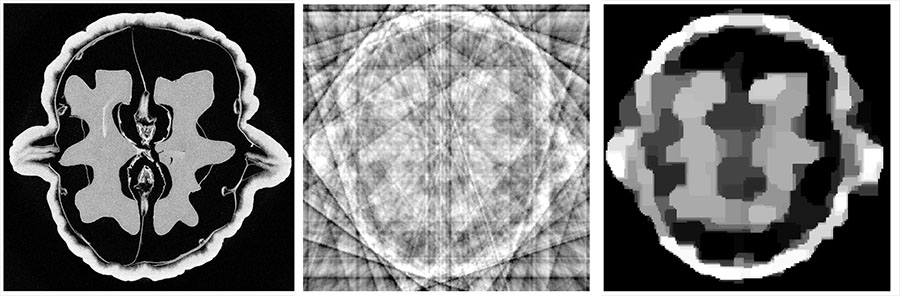
-Three-dimensional X-ray imaging (more information)
-Recovering the inner structure of the Earth based on earthquake measurements
-Reconstructing electric conductivity from current-to-voltage boundary measurements (see this page and this page)
-Finding cracks inside solid structures
-Prospecting for oil and minerals
-Monitoring underground contaminants
-Finding the shape of asteroids based on light-curve data (see this page)
The common features of all this problems are the need to understand indirect measurements and to overcome extreme sensitivity to noise and modelling inaccuracies.
What does the course contain?
The goals of the course are
- introduce discrete matrix models of some widely used measurements, such as tomography and convolution
- show how to detect ill-posedness (sensitivity to measurement noise) in matrix models using Singular Value Decomposition
- compute noise-robust reconstructions using regularization
- write Matlab algorithms for sharpening photographs and computing tomographic reconstructions
The lectures make up 10 credit units. In addition to lectures the course involves a project work. It is done in teams of two and gives 5 credit units to each student.
The course is in total 15 credit units.
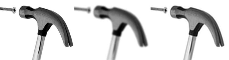
Left: original image. Middle: misfocused image. Right: sharpened image.
Lecturer
Assistants
Credit units
15 op.
Type
Advanced studies (syventävä opintojakso)
Prerequisites
Recommended courses to take before this course: Linear algebra 1 and 2, Applications of matrix computations.
Some previous experience with Matlab programming is very helpful. Tutorials for learning basics of Matlab are available for example at the following locations:
Project work
There are two project work topics: image deblurring and real-data X-ray tomography.
The idea is to study an inverse problem both theoretically and computationally in teams of two students. The end product is a scientific poster that the team will present in a poster session on Thursday, May 8, 2014 at 14-16in the Industrial Mathematics Laboratory (Exactum C131). The poster can be printed using the laboratory's large scale printer. The classical table of contents is recommended for structuring the poster:
1 Introduction
2 Materials and methods
3 Results
4 Discussion
Section 2 is for describing the data and the inversion methods used. In section 3 those methods are applied to the data and the results are reported with no interpretation; just facts and outcomes of computations are described. Section 4 is the place for discussing the results and drawing conclusions.
Here are more specific instructions concerning the two project work topics.
Image deblurring: think about an experiment where you can take three photos of the same object: sharp, a little blurred (misfocused) and a bit more blurred. The object should be essentially two-dimensional, such as text or image on paper or a coin. You can either take three separate photos using three different focus settings in the camera, or you can place three identical objects at three different distances from the lens. It is advisable that each object contains a small black dot on a white surface; this will give you an empirical point spread function. The aim of the project work is to implement and test a deblurring algorithm for the photographs and compare the final result to sharply photographed ground truth. You can choose the large-scale inversion method you want to use in the project. Preferably, take one of the following:
- matrix-free Tikhonov with the conjugate gradient method,
- matrix-free approximate total variation with the Barzilai-Borwein method.
If you plan to use some other method, discuss this plan with the lecturer in the First Goal meeting. Optimally, you should have an automatic method for choosing the regularization parameter and an automatic stopping criteria for the iteration. These are both difficult requirements, so have a simple approach as plan B if a more complicated approach does not work. Here is a used in previous years' courses, you can use it if you want. Also, here are extra instructions which you need not follow in detail: . Photographic data collection will be done on Friday, 4.4.2014, at 12:15-14:00 in the Industrial Mathematics Laboratory (Exactum C131).
X-ray tomography: Download the set of measured walnut . The dataset contains
- X-ray projection data in sinogram form,
- measurement matrix, and
- a filtered back-projection reconstruction from complete data for comparison.
In the project you are supposed to take a subset of the data with only few projections, such as 20 projection directions. Use one of these methods to recover the walnut slice from sparse data:
- Tikhonov regularization based on conjugate gradient method,
- approximate total variation regularization implemented iteratively with the Barzilai-Borwein method.
Optimally, you should have an automatic method for choosing the regularization parameter and an automatic stopping criteria for the iteration. These are both difficult requirements, so have a simple approach as plan B if a more complicated approach does not work.
First goal consists of two things: (a) two first sections should be preliminary written in LaTeX (not necessarily in poster format yet) and (b) the Matlab codes at the following webpages should be run and studied (only the page related to your topic):
Two things will be graded in the meeting about the first goal: (a) the draft of project work and (b) your understanding of the Matlab codes at the above webpage relevant to your topic. The grade represents 30% of the final grade of the project work. Please agree on a meeting time (in the period April 1-4) with the lecturer for reviewing and grading the first goal.
Second and final goal: poster is presented in the session on May 8. The poster will be printed in size A1. You may create your own poster (from scratch), or you can use e.g. as a starting point and edit its layout, colors, fonts, etc. as much as you like.
Please send your poster via email as a pdf attachment to Esa Niemi by Monday 5th May, 12 pm. Then your poster will be printed by the poster session on May 8.
The poster session will be held on Thursday, May 8, 14:15-15:30 in the Industrial Mathematics Laboratory (Exactum C131).
Lectures
Period III: Lectures as follows:
Tuesday 10-12 in room D123
Wednesday 12-14 in room D123
Friday 12-14 in room C123.
Two hours of exercise classes per week.
Period IV: Lectures and exercises in the beginning of the period. Later project work, which is reported as a poster in a poster session.
14.1.2014 Tuesday: Introduction to inverse problems. Specific problems discussed were , X-ray tomography, electrical impedance tomography and .
Lecture slides: , , .
Tomography videos: construction of the sinogram, reconstruction using Filtered Back-Projection.
Book sections (Mueller-Siltanen 2012): Chapter 1.
15.1.2014 Wednesday: Basics of one-dimensional convolution, including the continuous model and its matrix approximation.
Book sections (Mueller-Siltanen 2012): Sections 2.1.1. and 2.1.2.
Matlab codes: , , , , , , , .
21.1.2014 Tuesday: Analysis of 1-dimensional discrete deconvolution continues. Assessment of ill-posedness of convolution matrices using Singular Value Decomposition (SVD) and observing the decay of singular values to zero. Numerical experiments showing the failure of naive inversion. A first look at robust reconstructions based on truncated SVD.
Book sections: 2.1.3, 2.1.4, 3.5, 3.6.
Matlab codes: , , .
22.1.2014 Wednesday: Overview of the topics that will be covered in the course:
-Motivation using 1D deconvolution and 2D tomography
-Theory of inverse problems: existence, uniqueness, stability, and regularization
-Regularization methods: truncated SVD, Tikhonov regularization, total variation regularization
-Large-scale computation for practical problems using iterative techniques
After the overview we moved on to study the basics of X-ray attenuation and two-dimensional tomography. We studied the ill-posedness of tomography by looking at the singular values of tomography matrices. Also, naive inversion (based on least-squares solution) fails in the case of 2D tomography as it failed for 1D deconvolution. Finally, we had a second look at robust reconstructions based on truncated SVD.
Lecture slides:
Book sections: 2.3.1, 2.3.2, 2.3.4.
Matlab codes: , ,
, ,
, , , ,
, ,
Remarks about the codes:
- The routines need to be run in the above order for each value of n separately.
- You will need the image processing toolbox; otherwise the routine radon.m is not available for you.
- You need to have a subfolder called "data" in your working folder. That's where the data files of type ".mat" will be saved. The routine XRM1_matrix_comp.m actually creates the folder "data" automatically for you; if you run it again, Matlab may give you a warning that the directory already exists. You can ignore this warning.
- If you run the routine XRM3_NoCrimeData_comp.m with one value of n first and then with another value of n, there is an error message. I have no idea why. If you find the reason please let me know. Anyway, type "clear all" in Matlab after seeing the error message and you're good to go.
- Computing XRM5_SVD_comp.m can take a really long time when N is large (32 or bigger). For your convenience, I upload here a couple of SVD results: , .
24.1.2014 Friday: Introduction to the general framework of inverse problems. Least squares solution and minimum norm solution for matrix equations.
Lecture slides:
Book sections: 3.1, 3.4 and 4.1.
28.1.2014 Tuesday: Continuous model of one-dimensional convolution and deconvolution, including Fourier transform analysis.
Radon transform in X-ray tomography. Fourier slice theorem.
Lecture notes: , (the latter is in Finnish).
Book section: 2.3.3.
29.1.2014 Wednesday: Two different derivations of the Filtered Back-Projection (FBP) algorithm for X-ray tomography.
Complementary lecture notes are available .
This is the Matlab file created in the end of the lecture:
Book section: 2.3.3.
31.1.2014 Friday: Invisible structures in X-ray tomography. Interplay between continuous and discrete tomography. Introduction to Tikhonov regularization.
Lecture notes:
Book section 5.1.
4.2.2014 Tuesday: Tikhonov regularization continued. Derivation of normal equations. Writing the Tikhonov regularization task in stacked form.
Matlab file:
Book section 5.2.
5.2.2014 Tuesday: Generalized Tikhonov regularization and the corresponding normal equations. A few words and numerical examples about iterative solution of linear equations. The L-curve method for choosing the regularization parameter in Tikhonov regularization.
Matlab routines: , , , . For matrix-free iterative regularization of tomography, see this page and this page.
Book sections: 5.3, 5.4.2.
7.2.2014 Friday: Conjugate gradient method for large-scale Tikhonov regularization.
Book section: 5.5.
18.2.2014 Tuesday: Total variation regularization.
Book sections: 6.1 and 6.2.
Matlab resources: (note that Matlab Optimization Toolbox is needed)
19.2.2014 Wednesday: The S-curve method for sparsity-based determination of TV regularization parameter. Large-scale implementation of TV regularization via smoothing and Barzilai-Borwein minimization.
Book sections: 6.3 and 6.4.
Matlab resources (convolution, Matlab Optimization Toolbox needed):
,
Matlab resources (matrix-based tomography):
, , , ,
, , ,
Matlab resources (matrix-free large-scale tomography):
see this page.
14.3.2014 Friday: Home exam return session & project work assignment.
Exercises
Tuesday 16-18 in room D210 (Physicum)
Friday 14-16 in room C128 (Exactum)
You may choose which one of the exercise sessions you participate. The theoretical exercises (T1, T2, ...) should be done in advance and they will be checked in the beginning of the exercise session. The Matlab exercises (M1, M2, ...) as well as the LaTeX exercises (L1, L2, ...) can be done in advance or during the exercise session.
(January 21-24, 2014),
(January 28-31, 2014),
(February 4-7, 2014), , ,
(February 11-14, 2014), ,
(February 18-21, 2014), feel free to modify this file: (the routine will give an error message without appropriate modification).
Course Materials
The course follows the book Linear and Nonlinear Inverse Problems and Practical Applications by J.L. Mueller and S. Siltanen (SIAM 2012).
Part I of the book will be covered.
The book is available at Google books and at the SIAM bookstore.
Also, the relevant chapters of the book are available for copying in Exactum room C326. You can now also find chapters 6 and 9 from the copy room.
The Matlab codes used in the book are collected to this page.

Exam
The answers to the exam questions should be returned in the examination session on Friday, March 14, 2014, at 12:15. The hall is Exactum C123.
More instructions are given in the exam itself: .
Here is the draft report file for Problem 3: .
Matlab resources:
Registration
Did you forget to register? What to do?