Inverse problems, spring 2015
Inverse problems, spring 2015
The course is lectured in English
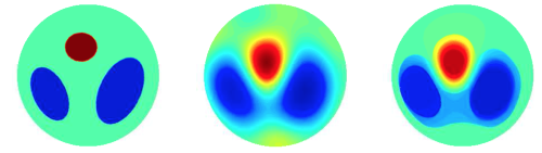
Figure: electrical conductivity distribution (left), nonlinear reconstruction from voltage-to-current boundary measurements (middle), edge-enhanced nonlinear reconstruction (right).
Inverse problems are about interpreting indirect measurements. The scientific study of inverse problems is an interdisciplinary field combining mathematics, physics, signal processing, and engineering. Examples of inverse problems include
- Three-dimensional X-ray imaging (more information, also see this video and this video)
- Recovering the inner structure of the Earth based on earthquake measurements
- Sharpening a misfocused photograph (more information )
- Reconstructing electric conductivity from current-to-voltage boundary measurements (see this page and this page)
- Finding cracks inside solid structures
- Prospecting for oil and minerals
- Monitoring underground contaminants
- Finding the shape of asteroids based on light-curve data (see this page)
The common features of all this problems are the need to understand indirect measurements and to overcome extreme sensitivity to noise and modelling inaccuracies.
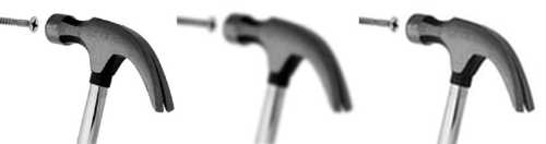
Figure: sharp image (left), misfocused image (middle), sharpened image by deconvolution (right).
Inverse problems research is an active area of mathematics.
At the Department of Mathematics and Statistics the field is represented by three research groups belonging to
a Centre of Excellence of Academy of Finland:
What does the course contain?
The goals of the course are
- introduce discrete matrix models of some widely used measurements, such as tomography and convolution
- show how to detect ill-posedness (sensitivity to measurement noise) in matrix models using Singular Value Decomposition
- compute noise-robust reconstructions using regularization
- write Matlab algorithms for sharpening photographs and computing tomographic reconstructions
- discussion of nonlinear inverse problems, with Electrical Impedance Tomography as an example
The course involves working with practical measurement data. Therefore, it is a good choice for students planning a career in industry.
The lectures make up 10 credit units. In addition to lectures the course involves a project work. It is done in teams of two and gives 5 credit units to each student.
The course is in total 15 credit units.
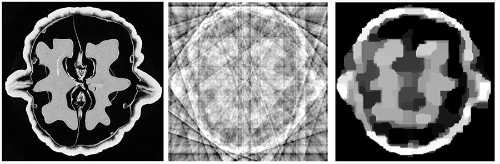
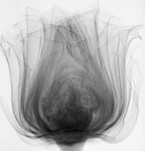
Figure: high-resolution X-ray tomographic slice through a walnut (left), reconstruction from few data using an old method (middle), and reconstruction from few data using a modern method (right).
Lecturers
Main lecturer: Samuli Siltanen
Guest lecturers: Paola Elefante, Andreas Hauptmann, Alexander Meaney, and Zenith Purisha
Scope
15 sp.
Type
Advanced studies
Prerequisites
Recommended courses to take before this course: Linear algebra 1 and 2, Applications of matrix computations.
Some previous experience with Matlab programming is very helpful.
Structure of the course
Period III: Lectures as follows:
Tuesday 10-12 in room D123
Wednesday 12-14 in room D123
Friday 12-14 in room C123.
Two hours of exercise classes per week.
Period IV: Project work, which is reported as a poster in a poster session.
Lectures
Lecture 1 (January 13, 2015)
Introduction to inverse problems, indirect measurements and ill-posedness.
The (huge) files of the presentations are available in this Dropbox folder.
The practical information slides are available in the file .
Lecture 2 (January 14, 2015)
One-dimensional convolution of real-valued functions. Book section 2.1.1.
Matlab resources: , , , , .
Lecture 3 (January 16, 2015)
One-dimensional convolution in both continuous and discrete form. First example of the failure of naive inversion in the case of an ill-posed problem. Book sections 2.1.2 and 2.1.3.
Matlab resources: , , ,
, , ,
Lecture 4 (January 20, 2015)
Computational studies of the one-dimensional deconvolution. Simulation of crime-free data. Book sections 2.1.3 and 2.1.4.
Lecture 5 (January 21, 2015)
Singular value decomposition of matrices and how it explains the instability of naive inversion. Book chapter 3.5.
Matlab resources: , , ,
Lecture 6 (January 23, 2015)
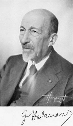
Well-posedness and ill-posedness in the sense of Hadamard. Quick introduction to the concept of regularization. Minimum norm solution and the Moore-Penrose pseudoinverse. Book sections 3.1 and 3.4. and 4.1. (No computational stuff this time.)
Lecture 7 (January 27, 2015)
Introduction to X-ray measurements and their mathematical modelling. Book sections 2.3.1, 2.3.2 and 2.3.4.
Videos: Recording a projection image by scanning, Collection of tomographic data
Lecture 8 (January 28, 2015)
Construction of X-ray measurement matrices using Matlab's built-in function radon.m. Naive reconstruction from data with inverse crime. Also: truncated SVD reconstructions from data with inverse crime. Book sections 2.3.4, 2.3.5, 4.2 and 4.4.3.
Matlab resources: , , ,
Lecture 9 (January 30, 2015)
Two demonstrations of current research in X-ray tomography reconstruction methods.
Paola Elefante: Dynamic X-ray sparse tomography
Motivation for sparse tomography: hints on how cancer is formed and X-rays as environmental factors, possible improvements for medical care. Motivation for dynamic tomography: veterinary applications, material testing, monitoring the effects of cancer medications, and angiography (with video). The level set method, brief introduction. Presenting simulated data, comparison with FBP and Tikhonov. State of the art of local research and upcoming challenges. Slides available here.
Zenith Purisha: X-ray tomography using MCMC and NURBS
1. Motivation for using NURBS, the building blocks in CAD modelling. Why does CAD use NURBS: it involves a few parameters only, making computation efficient. Taking sparse data from a homogenous object to have quick measurement process. In medical environment, sparse data will reduce radiation dose. The idea is implementing Bayesian Inversion and NURBS to recover the parameters.
2. Introduction about NURBS (one slide, a video), Tomographic Measurement model (Included Basic Xray measurement, Radon transform, Discrete tomographic Data, and of course NURBS-based tomographic model), Bayesian Inversion and MCMC.
3. Results of reconstruction from real data
Lecture 10 (February 3, 2015)
Construction of tomographic data without inverse crime. The trick is to simulate the sinogram at higher resolution and then interpolate from that the sinogram corresponding to lower resolution.
Matlab resources: ,
Lecture 11 (February 4, 2015)
Introduction to Tikhonov regularization. Finding the minimum of the Tikhonov functional using the singular value decomposition.
Book section 5.1.
Matlab resources: ,
Lecture 12 (February 6, 2015)
Introduction to the generation of X-rays. Tomography lab visit.
Lecture 13 (February 10, 2015)
Introduction to normal equations and the stacked form method for computing Tikhonov regularized solutions.
Matlab resources: ,
Book section 5.2.
Lecture 14 (February 13, 2015)
Large-scale implementation. Matrix free formulation and the conjugate gradient method. Book section 5.5
Matlab resources: , ,
Further reading material on optimization and conjugate gradient can be found here: http://www4.ncsu.edu/~ctk/lv/lvpub.html
Lecture 15 (February 17, 2015)
Sparsity-promoting reconstruction for the deconvolution problem using L1-norm regularization. Book sections 6.1 and 6.2.
Lecture 16 (February 18, 2015)
Review of four variational regularization methods in the case of 1D deconvolution:
(1) Classical Tikhonov regularization (penalty: L2 norm of f),
(2) Generalized Tikhonov regularization with derivative penalty (penalty: L2 norm of Lf),
(3) Sparsity-promoting regularization (penalty: L1 norm of f),
(4) Total variation (TV) regularization (penalty: L1 norm of Lf).
Implementation of TV regularization for the 2D tomography case using quadratic programming. Book section 6.
Matlab resources for 1D deconvolution: all files updated, please download them from this Dropbox directory.
Matlab resources for 2D tomography: (it works!)
Lecture 17 (February 20, 2015)
Closer study of TV-based tomography using the routine . We added comparison to filtered back-projection, as you can see by running . You will need the additional files and . Discussion of large-scale TV computation based on smoothing out the absolute value function and applying the Barzilai-Borwein minimization method for the resulting smooth objective functional.
Book section 6.
For a basic introduction to optimization, see Chapter 10 of the classical book Numerical Recipes.
Lecture 18 (February 24, 2015)
Wavelet-based regularization and Besov norm penalties. See .
Book chapter 7.
Matlab resources: , , , .
Lecture 19 (February 25, 2015)
Mathematical derivation of the Filtered Back-Projection method. Here are details: . Also, see Chapter 3 of the book by Kak and Slaney.
Book chapter 2.3.3.
Lecture 20 (Last lecture! February 27, 2015)
Introduction to the course exam. It is recommended to take part in this session if you plan to pass the course.
Discussion of project work topics, division to project groups. It is recommended to take part in this session if you plan to make the project work.
Matlab resources
You can always find the latest set of Matlab files in this Dropbox directory.
Exam
The home exam is . Please return your answers at latest on March 16 by email attachment to Andreas Hauptmann. Specific instructions are given in the exam itself.
Exam files: , ,
Bibliography

Exercises
Course assistant: Andreas Hauptmann
The exercise sessions will be held in the computer room C128. There are two sessions:
Tuesday 12-14
Thursday 14-16
The theoretical exercises are to be presented by the students. In each session the students mark the exercises they have completed and according to this list one student will be chosen per exercise to present.
The Matlab exercises will be checked individually at the computers present. The Matlab exercises can be completed in pairs of two. Both students have to be present and able to explain the code.
Points for all completed exercises will be accumulated and part of the final grade.
NOTE! It has been decided that we will not publish the solutions for future exercises. Please attend the exercise sessions and/or ask your fellow students.
(January 20-22, 2015)
(January 27-29, 2015)
(February 3-5, 2015)
(February 10-12, 2015)
(February 17-19, 2015) - M1 & M2 corrected
(February 24-26, 2015)
Project work
Project work assistants: Alexander Meaney and Andreas Hauptmann
The idea is to study an inverse problem both theoretically and computationally in teams of two students. The end product is a scientific poster that the team will present in a poster session on
 Thursday, May 7, 2015 at 14:15-16:00 in the Industrial Mathematics Laboratory (Exactum C131).
The poster can be printed using the laboratory's large scale printer. Please send your poster via email as a pdf attachment to Andreas Hauptmann by Tuesday 5th May, 12 pm. Then your poster will be printed by the poster session on May 7.
The idea of the project work is to study an inverse problem both theoretically and computationally in teams of two students. The end product is a scientific poster that the team will present in a poster session in the Industrial Mathematics Laboratory. The poster can be printed using the laboratory's large scale printer. The classical table of contents is recommended for structuring the poster:
1 Introduction
2 Materials and methods
3 Results
4 Discussion
Section 2 is for describing the data and the inversion methods used. In section 3 those methods are applied to the data and the results are reported with no interpretation; just facts and outcomes of computations are described. Section 4 is the place for discussing the results and drawing conclusions.
The project is about X-ray tomography. You can measure a dataset yourself in the X-ray facility of the Industrial Mathematics Laboratory:
You can choose your own object to image in the X-ray lab. Examples of good objects include a capasitor, excised tooth, or other objects of roughly the size of a fingertip. Please contact Alexander Meaney to find out if your object is good for imaging.
In the project you are supposed to take a subset of the data with only few projections, such as 20 projection directions. It's a good idea to use one of these methods:
- Tikhonov regularization based on conjugate gradient method, perhaps with non-negativity constraint,
- approximate total variation regularization implemented iteratively with the Barzilai-Borwein method.
Optimally, you should have an automatic method for choosing the regularization parameter and an automatic stopping criteria for the iteration. These are both difficult requirements, so have a simple approach as plan B if a more complicated approach does not work.
First goal consists of two things: (a) two first sections should be preliminary written in LaTeX (not necessarily in poster format yet) and (b) the Matlab codes at the following webpage should be run and studied:
Two things will be graded in the meeting about the first goal: (a) the draft of project work and (b) your understanding of the Matlab codes at the above webpage relevant to your topic. The grade represents 30% of the final grade of the project work. Please agree on a meeting time (in the period April 1-4) with the lecturer for reviewing and grading the first goal.
Second and final goal: poster is presented in the session on May 7. The poster will be printed in size A1. You may create your own poster (from scratch), or you can use e.g. this template as a starting point and edit its layout, colors, fonts, etc. as much as you like.
Results of the poster projects
The posters have been presented in a poster session on May 7. Each group had 5 minutes to present their project and explain what they have done. The resulting posters can be found as PDF files in the following:
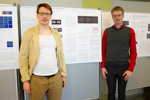
And here are some happy students presenting their work. The pictures have been taken during the poster session.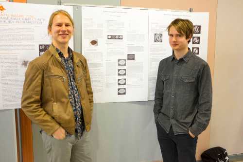
Feedback
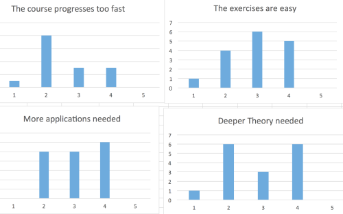
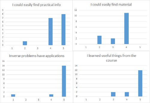
Feedback was collected in the middle of the course using .
Here are the results:
- I strongly disagree
- I somewhat disagree
- No opinion
- I agree to some extent
- I strongly agree