Bayesian inversion, spring 2016
Bayesian inversion, spring 2016
 Please send the poster file to zenith.purisha@helsinki.fi before 18 May 2016. The posters will be printed and you may take it on Thursday at 9 am in C131. The poster presentation is from 9-11, but let them there to be seen by others until 4 pm.
Teacher: Tapio Helin ja Samuli Siltanen
Scope: 15 cr
Type: Advanced studies
Teaching: Lectures, exercises, and project work with measured data
Topics: Theory and computational methods of Bayesian inversion
Prerequisites for the theoretical part: Measure and integration theory
Prerequisites for the computational part: Basics of mathematical probability, some Matlab skills such as given by course Applications of matrix computations
The [toc] macro is a standalone macro and it cannot be used inline. Click on this message for details.
Inverse problems are about interpreting indirect measurements. The scientific study of inverse problems is an interdisciplinary field combining mathematics, physics, signal processing, and engineering. Examples of inverse problems include
- Three-dimensional X-ray imaging (more information, also see this video and this video)
- Recovering the inner structure of the Earth based on earthquake measurements
- Sharpening a misfocused photograph ( more information )
- Reconstructing electric conductivity from current-to-voltage boundary measurements (see this page and this page )
- Finding cracks inside solid structures
- Prospecting for oil and minerals
- Monitoring underground contaminants
- Finding the shape of asteroids based on light-curve data (see this page )
The common features of all this problems are the need to understand indirect measurements and to overcome extreme sensitivity to noise and modelling inaccuracies.
The topic of the course is statistical inverse problems. The lectures consist of two parts:
Theoretical modelling in Bayesian inverse problems (Tapio Helin)
Computational methods (prof. Samuli Siltanen)
The goals of the course are
(computational part)
- introduce the framework for statistical Bayesian inverse problems
- understand main ideas of uncertainty quantification via the Bayes formula
- learn efficient computational methods for exploring the posterior distribution.
In particular, two central Markov chain Monte Carlo algorithms are studied and implemented in Matlab: Metropolis-Hastings algorithm and the Gibbs sampler.
(theoretical part)
- learn the general Bayes formula
- show well-posedness of Bayesian inverse problems
- study continuity properties of the solution when discretization is refined
News
Teaching schedule
Period III: Lectures as follows:
Wednesday 10-12 in room C124 Thursday 10-12 in room B120 Friday 10-12 in room C124.
Two hours of exercise classes per week.
Period IV: Lectures continue as long as needed (but not for the whole period). There is a project work, which is reported as a poster in a poster session in May. The exact date will be decided later.
Lectures
Wednesday 27.1.2016 Samuli Siltanen
Introduction to inverse problems and Bayes formula. Motivating examples: X-ray tomography and Glottal Inverse Filtering (GIF). Practical information about the course.
Introductory lecture slides (PDF)
Thursday 28.1.2016 Samuli Siltanen
Real-valued random variable, probability density function, and computational sampling.
Friday 29.1.2016 Tapio Helin
Motivation, sigma-algebras, Radon-Nikodym derivative and conditional expectation.
Wednesday 3.2.2016 Tapio Helin
Conditional expectation and probability continued, Bayes formula.
Thursday 4.2.2016 Tapio Helin
Proof of Bayes formula, some principals of Bayesian inference, example with Gaussian prior and noise.
First version of the lecture notes from the theoretical part:
Friday 5.2.2016 Samuli Siltanen
Conditional probability in the case of probability density functions. Linear measurement model.
The newest version of the lecture note is here:
The complete package including Matlab and LaTeX files is here:
Wednesday 10.2.2016 Tapio Helin
Gaussian posterior, Posterior consistency in over/underdetermined systems
Thursday 11.2.2016 Samuli Siltanen
Introduction of one-dimensional convolution as a measurement model leading to ill-posed inverse problems.
Here are the discrete convolution demonstration slides (with source files in the zip folder): , .
Here is the explanation regarding continuous and discrete model: .
We started building a Matlab library for studying one-dimensional convolution and deconvolution.
, ,
,
,
,
Friday 12.2.2016 Samuli Siltanen
Singular Value Decomposition (SVD) for matrices. Detecting ill-posedness. See the document .
Computation of SVD for the 1D convolution problem:
,
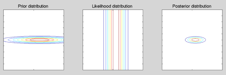
Illustration of Gaussian likelihood, prior and posterior distributions in a 2-dimensional toy example:
Wednesday 17.2.2016 Tapio Helin
Posterior consistency in underdetermined systems, metrics on probability space
Thursday 18.2.2016 Samuli Siltanen
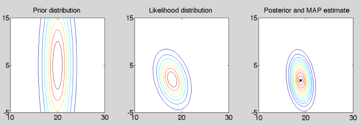
Definition and discussion of CM and MAP estimates. Derivation of a formula for the MAP estimate in the case of a Gaussian posterior (note that in that case the CM and MAP estimates are the same).
Introduction of a simple 2-dimensional example. It is a measurement scenario with two temperatures. Indoor temperature f1 is measured with thermometer T1 inside without connection to outdoor temperature. The outdoor temperature f2 is measured with thermometer T2, located in the windowpane. The reading of thermometer T2 is a linear combination of indoor and outdoor temperatures. Both thermometers are corrupted by additive Gaussian noise with standard deviation sigma. The prior is Gaussian. This Matlab file shows the situation:
Newest version of the notes:
Friday 19.2.2016 Samuli Siltanen
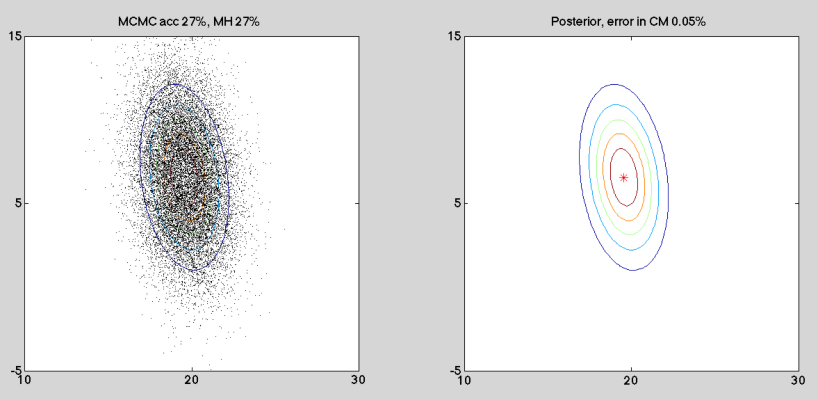
Markov chain Monte Carlo sampling using a simple Metropolis-Hastings method.
For explanation of the Metropolis-Hastings method, see Section 5.3.3 of the old lecture note .
The two-dimensional example of measuring indoor and outdoor temperatures using two thermometers is here in a revised form:
, ,
Wednesday 24.2. Guest Lecturer: Dr. Marko Laine (Finnish Meteorological Institute)
The slides of the first part:
And the MCMC toolbox can be found here: http://helios.fmi.fi/~lainema/mcmc/
Thursday 25.2. Tapio Helin
Hellinger distance of two Gaussians, well-posedness of the posterior with perturbed measurement and prior
Friday 26.2. Tapio Helin
Well-posedness of the posterior with perturbed prior continued, introduction to probability in Banach spaces
Newest version of the notes:
Wednesday 2.3. Tapio Helin
Introduction to probability in Banach spaces, Gaussian random variables
Thursday 3.3. Samuli Siltanen
MCMC computation using the Gibbs sampler.
Matlab file:
Friday 4.3. Tapio Helin
Gaussian random variables, Fernique theorem, Cameron-Martin space
Wednesday 16.3. Samuli Siltanen
Computation of MAP estimates for the 1D deconvolution problem. We use several choices of priors.
Newest version of the lecture notes: , see the new chapter 2.7.
Matlab routines used in the lecture (some of these are posted again here in the same form than above):
, ,
,
,
,
,
Thursday 17.3. Samuli Siltanen
Computation of CM estimates for the 1D deconvolution problem. We use the Metropolis-Hastings algorithm with several choices of priors.
Matlab routines:
,
,
Friday 18.3. Samuli Siltanen
Practicalities about the project work:
- forming the teams (two students in each team)
- discussion of the two-phase structure of the project work
- choosing the topics of the project work, involving real data measurement (tomography, photographic, other)
- agreeing upon the mid-project deadline
- setting the date for the final poster session
Wednesday 23.3. Tapio Helin
Cameron-Martin spaces, stability of Bayesian inversion for non-linear problems
The newest version of the lecture note is here:
Thursday 31.3. Tapio Helin
Stability and approximation properties
Friday 1.4. Tapio Helin
Bayesian inversion for the inverse heat equation
The final version of the lecture notes:
Exams
Deadline for returning answers is 12 o'clock noon on Monday, April 25, 2016.
Course material
Lecture notes will be updated here as the course progresses.
The book Mueller&Siltanen: Linear and nonlinear inverse problems with practical applications (SIAM 2012) explains the computational models used in the course. These lecture notes cover pretty much everything in the computational part: .
For the theoretical part we partly use the lecture notes by Masoumeh Dashti and Andrew Stuart. Also, an excellent review on Bayesian inverse problems in Banach spaces is available in this paper by Andrew Stuart (only available on UH network).
A slide with preliminaries and a few basics about probability distributions (in particular Gaussian) from the lecture Statistical Inverse Problems at the University of Eastern Finland: , (We thank Janne Huttunen and Ville Kolehmainen for providing the slides).
Some courses in Inverse Problem in Imaging and one of Bayesian Inversion lectures: .
Registration
Did you forget to register? What to do?
Exercises
Teaching assistants: Andreas Hauptmann & Zenith Purisha
Assignments
The assignments are to be prepared for the exercise class, where the students are expected to present the solutions.
- (Due 09.02.),
- (Due 16.02.), files needed: , , , ,
- (Due 23.02.), One suggested homework: (Take this as suggestion, not as model solution!)
- (Due 01.03.), files needed: . Solution codes:
- (Due 15.03)
- (Due 22.03), files needed: , , ,
Exercise classes
Tuesday 10-12: 09.02.2016 - classic - C124
Tuesday 10-12: 16.02.2016 - computer - C128
Tuesday 10-12: 23.02.2016 - classic - C124
Tuesday 10-12: 01.03.2016 - computer - C128
Tuesday 10-12: 15.03.2016 - classic - C124
Tuesday 10-12: 22.03.2016 - computer - C128
Tuesday 10-12: 05.04.2016 - computer - C128 (Last exercise session: we go through computational measurement models needed in the project works.)
Project work
Project work assistants: Andreas Hauptmann and Zenith Purisha.
The idea is to study a Bayesian inverse problem both theoretically and computationally in teams of two students. The end product is a scientific poster that the team will present in a poster session on May 19 (at 9-11, Exactum first floor corridor). The poster can be printed using the large-scale printer of the Industrial Mathematics Laboratory.
The classical table of contents is recommended for structuring the poster:
1 Introduction
2 Materials and methods
3 Results
4 Discussion
Section 2 is for describing the data and the inversion methods used. In section 3 those methods are applied to the data and the results are reported with no interpretation; just facts and outcomes of computations are described. Section 4 is the place for discussing the results and drawing conclusions.
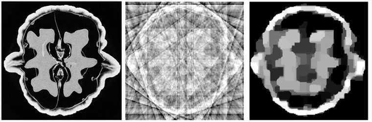
The recommended measurement context of the project is X-ray tomography. You can measure a dataset yourself in the X-ray facility of the Industrial Mathematics Laboratory:


The project work has two phases, each with a specific goal.
First goal (deadline April 15) consists of two things: (a) two first sections should be preliminary written in LaTeX (not necessarily in poster format yet) and (b) the Matlab codes related to the measurement should be run and studied. Two things will be graded in the meeting about the first goal: (a) the draft of project work and (b) your understanding of the available Matlab codes relevant to your topic. The grade represents 30% of the final grade of the project work. Please agree on a meeting time with the lecturer for reviewing and grading the first goal.
Second and final goal (deadline May 19): poster is presented in the poster session. The poster will be printed in size A1. You may create your own poster (from scratch), or you can use e.g. this template as a starting point and edit its layout, colors, fonts, etc. as much as you like.
Example posters are shown on this page.
Course feedback
Course feedback can be given at any point during the course. Click here.