Inverse problems, spring 2017
Inverse problems, spring 2017
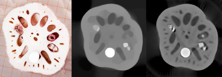
Question: What on earth is this picture about?
Answer: It is an example of X-ray tomography! See this video. And this page.
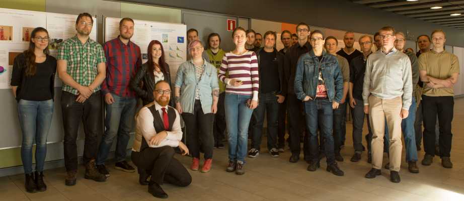
Class of 2017 (poster session):
Teacher: Samuli Siltanen
Scope: 15 cr (lecture part and project work combined)
Type: Advanced studies
Teaching:
Topics: Inverse problems are about measuring something indirectly and trying to recover that something from the data. For example, a doctor may take several X-ray images of a patient from different directions and wish to understand the three-dimensional structure of the patient's inner organs. But each of the 2D images only shows a projection of the inner organs; one has to actually calculate the 3D structure using a reconstruction algorithm. This course teaches how to
- model a (linear) measurement process as a matrix equation m = Ax + noise,
- detect if the matrix A leads to an ill-posed inverse problem,
- design and implement a regularized reconstruction method for recovering x from m. We study truncated singular value decomposition, Tikhonov regularization, total variation regularization and wavelet-based sparsity,
- measure tomographic data in X-ray laboratory,
- report your findings in the form of a scientific poster.
See this page for more information about inverse problems.
Here are the old homepages of this course: 2015, 2014, 2013. This year the course is roughly the same than in those past years.
Prerequisites: Linear algebra, basic Matlab programming skills, interest in practical applications, and a curious mind. The course is suitable (and very useful) for students of mathematics, statistics, physics or computer science.


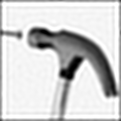
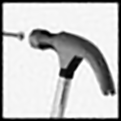
Consider the above photographic situation. You would like to have taken the left image: sharp and beautiful. However, due to misfocusing and high ISO setting in the camera, you ended up with the blurry and noisy picture on the right. Is there any chance to save the day? Well, one can apply deblurring, one of the topics of this course. Below you see three different deblurring methods with varying success. From left to right: basic regularization, total variation, and total generalized variation. (Thanks to Professor Kristian Bredies for sharing his amazing TGV algorithm!)

News
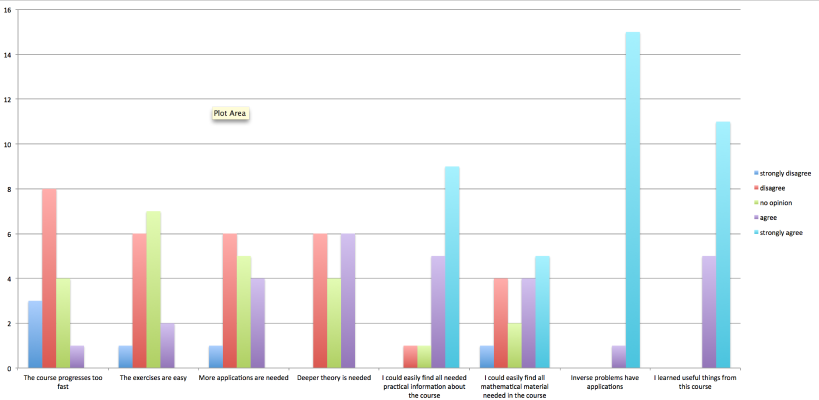
Results of the mid-course questionnaire (Feb 15). It seems that all is going pretty well in general. Let's discuss in the lecture about how to make finding material easier.
Lecture 16 (March 24)
Project work info. The goals of this session are
- Dividing students into project teams of two members each,
- Choosing the topic (tomography or deconvolution data, what is the focus of the project, what methods to try),
- Understanding the goals of Phase 1 and Phase 2 of the project,
- Agreeing on meeting times for reviewing Phase 1 of the projects.
Lecture 15 (March 22)
Real-data X-ray tomography. How to go from projection images to line integral data? What are the crucial properties of the variants of tomography, such as limited-angle, region-of-interest, sparse and exterior tomography?

Lecture, part 1/2 (screen capture)
Lecture, part 2/2 (screen capture)
Lecture 14 (March 17)
Choosing the regularization parameter. There are several methods, applicable to more or less of the different regularization approaches.
- L-curve method (mainly for Tikhonov)
- Morozov discrepancy principle (Tikhonov, has been extended to TV in recent research from Hong Kong)
- S-curve method (for sparsity-promoting regularization)
- Multi-resolution consistence method (for TV, see this file)
We will take a look of these methods and test some of them.
Lecture, part 1/2 (screen capture)
Lecture, part 2/2 (screen capture)
Lecture 13 (March 15)
Wavelet transform in dimensions 1 and 2. Large-scale sparsity-promoting reconstruction with Iterative Soft Thresholding Algorithm (ISTA).
 Matlab resources:
Lecture, part 1/2 (screen capture)
Lecture, part 2/2 (screen capture)
Lecture 12 (Friday, March 3)
Planning the remaining lectures of the course. We used the "double team" brainstorming method and ended up with this set of suggestions:
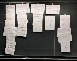
The results of the planning are seen in the themes for lectures 13, 14 and 15 above.
Wednesday, March 1. The lecturer is sick (damn this flu season!).
Instead of the lecture, please read Section 3.2 of this note on the Haar wavelet transform:
Study these Matlab routines and clarify to yourself how the codes and the text are connected.
Matlab resources:
Lecture 11 (February 24)
Recap of the construction of the tomographic "rectangle" phantom. Simulating tomographic data with no inverse crime, using higher-resolution simulation and interpolation. Applying
- Truncated SVD (TSVD),
- Tikhonov regularization, and
- Total Variation regularization
for the sparse-angle tomographic problem. Note that the Tikhonov regularization code above is written in a matrix-free fashion using the Conjugate Gradient (CG) method. We will talk about CG and other iterative solvers later in the course. The Total Variation computation is a two-dimensional adaptation of the quadratic programming formulation including inequality and equality constraints.
The files MyDS2.m and MyDScol.m are simple routines for downsampling an image by a factor of two.
See Sections 2.3, 4.4, 5.5, 6.2 and 5.2 in the book Mueller-Siltanen (2012).
Matlab resources:
Lecture, part 1/2 (screen capture)https://www.youtube.com/watch?v=x0wNtc9ZsRM&index=18&list=PL5vSJKR6SrD9124QEgO3_h1VPFgjG2lSQLecture, part 2/2
THERE IS NO LECTURE on Wednesday, February 22. The lecturer is traveling.
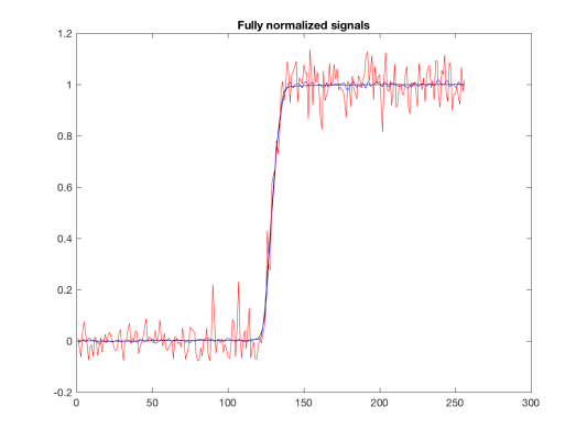
Instead of the lecture, please run all the Matlab files given below related to Lecture 10 using this year's target signal AND with the photographic data collected in Lecture 9.
Lecture 10 (February 17)
Discussed were three forms of variational regularization: Tikhonov, generalized Tikhonov and Total Variation regularization. We focused on the one-dimensional convolution model and used a simple finite-difference matrix L in the regularization terms.
Matlab demonstrations were based on the routines developed in the 2015 Inverse Problems course. They are given below. I recommend you to run them through with this year's target and with the photographic data collected in Lecture 9.
Note that whenever you change the dimension n of the unknown, you need to run deconv2_discretedata_comp.m, deconv3_naive_comp.m, deconv4_SVD_comp.m and deconv5_truncSVD_comp.m before running any of the Tikhonov or TV routines.
Matlab resources:
Lecture, part 1/3
Lecture, part 2/3
Lecture, part 3/3 (screen capture)
Lecture 9 (February 15)
Photographic data with varying levels of blur (from defocusing of the lens) and noise (from increasing the ISO) as measurements.
We photographed printouts of these two pictures posted to the wall:

Further, we picked out rows from the edge image and analysed the pixels values in Matlab.
Here are the two edge images we shot and processed:
Matlab resources:
Lecture, part 1/4
Lecture, part 2/4
Lecture, part 3/4 (screen capture)
Lecture, part 4/4 (screen capture)
Lecture 8 (February 10)
Naive inversion for non-square matrices. More precisely, we studied the case when A is a k x n matrix with k>n and when all the singular values of A are strictly positive. In that case there is a unique least-squares solution f0 to the equation m = Af. Further, we have f0 = inv(A^T A) A^T m.
See Sections 4.1 and 5.2 in the book Mueller-Siltanen (2012).
Matlab resources:
Here's the "video proof" about the minimum claim
Lecture, part 1/4
Lecture, part 2/4 (screen capture)
Lecture, part 3/4
Lecture, part 4/4
Lecture 7 (February 8)
Building the computational model Af=m for the 2D tomography problem. That is,
-designing a phantom for test cases (we went for three rectangles in empty background in the unit square), called SqPhantom.m,
-constructing and saving the matrix A for a selection of sizes of f and collections of X-ray projection directions,
-calculating and saving the Singular Value Decomposition for the matrix A.
Also, we tried out Truncated Singular Value Decomposition (TSVD) for robust reconstruction.
Matlab resources:
Lecture, part 1/5
Lecture, part 2/5
Lecture, part 3/5 (screen capture)
Lecture, part 4/5 (screen capture) Lecture, part 5/5 (screen capture)
Lecture 6 (February 3)
Recap of the trinity
(1) measurement data vector given by a device,
(2) continuum model of the physical measurement process, and
(3) computational model used in practical inversion.
The aim is to build two different example models, namely 1D deconvolution and 2D tomography. These two cases will be used throughout the course.
Construction of a matrix model m=Af using Matlab's radon.m routine. The matrix is constructed column by column by applying radon.m consecutively to unit vectors. While computationally inefficient, this approach provides an easy way for constructing system matrices for tomographic problems. The matrix A can then be studied by, for example, singular value decomposition.
Matlab resources:
Lecture 5 (February 1)
The lecturer is down with the flu and lost his voice! So the lecture is cancelled.
Instead of the lecture, please open the following page:
Read these items:
- Background and Applications
- Mathematical Model of X-ray Attenuation
- Tomographic Imaging with Full Data
- Tomographic Imaging with Sparse Data
The most important is "Tomographic Imaging with Sparse Data."
Also, please read Section 2.3 of the textbook (Mueller&Siltanen 2012).
Lecture 4 (January 27)
Building a simulated continuum model for 1D convolution in Matlab. See Section 2.1.1 in the book Mueller-Siltanen (2012).
Matlab resources:
,
,
,
,
,
,
,
,
Lecture 3 (January 25)
Quick look at the first noise-robust reconstruction method of the course: truncated singular value decomposition (TSVD).
We test TSVD with the simple convolution example from Lecture 2. Book chapters: 2.1, 4.2 and 4.1.1.
First observation about TSVD: the reconstruction is always a linear combination of singular vectors. Singular vectors are columns of the matrix V appearing in the singular value decomposition.
Second observation about TSVD: if we use only very few singular values, the reconstruction is not very accurate but extremely robust against noise. This means that the reconstruction does not change much form measurement to measurement even when there is large random noise added to the data.
Third observation about TSVD: it is not clear how to choose the truncation index r_\alpha in general. This is indeed a hard problem, and we will see some approaches to that later in the course.
Also, we started to discuss the difference between the continuum model for convolution (book chapter 2.1.1) and discrete model for convolution (book chapter 2.1.2).
Matlab resources:
Screen capture video 1/2, Screen capture video 2/2
Lecture 2 (January 20)
Discrete convolution between two vectors. How noise is amplified in naive inversion attempts. Book chapters: 2.1.
Lecture material: ,
Matlab resources:
Lecture 1 (January 18)
Introduction to inverse problems. Practicalities about the course.
Lecture material:
 Project work
Sign-up form for x-ray measurements: https://beta.doodle.com/poll/96rrp5ztg2psgmwm
Kick-off session on March 24 (usual lecture time and place): be there to get specific project work information.
Phase 1 review interviews will take place in the time period April 5-7. Be sure to agree on a time slot with the lecturer!
Phase 2 final goal is the Poster session on Friday, May 5, at 10-12 in the Exactum 1st floor hallway.
Project work assistants: Alexander Meaney, Zenith Purisha and Markus Juvonen.
The idea is to study an inverse problem both theoretically and computationally in teams of two students. The end product is a scientific poster that the team will present in a poster session on May 5 (details above).
The poster can be printed using the laboratory's large scale printer. Please send your poster via email as a pdf attachment to Markus Juvonen by Wednesday, 3rd May, 12 pm. Then your poster will be printed in time for the poster session.
The idea of the project work is to study an inverse problem both theoretically and computationally. The classical table of contents is recommended for structuring the first phase report and the poster:
1 Introduction
2 Materials and methods
3 Results
4 Discussion
Section 1 should briefly explain the topic in a way accessible to a non-expert.
Section 2 is for describing the data and the inversion methods used.
In section 3 the methods of Section 2 are applied to the data described in Section 2, and the results are reported with no interpretation; just facts and outcomes of computations are described.
Section 4 is the place for discussing the results and drawing conclusions.
The project is either about X-ray tomography or digital image processing. You can measure a dataset yourself in the Industrial Mathematics Laboratory.
X-ray topic: you can choose your own object to image in the X-ray lab. We can offer a range of tried-and-tested objects and tools to tailor them to your liking. Also, you can come up with your own idea of the measured object. The size of the object should not much exceed the size of an egg, and the chemical composition is important as X-ray attenuation contrast arises from electron densities in the materials. Please contact Alexander Meaney to find out if your object is good for imaging.
Photographic topic: take blurred or noisy photos of suitable targets.
In the project you are supposed to apply some of the regularization methods discussed in the course. Optimally, you should have an automatic method for choosing the regularization parameter and an automatic stopping criteria for the iteration. These are both difficult requirements, so have a simple approach as plan B if a more complicated approach does not work. Also, when choosing your objects of measurement, it's good to think about mathematical models of a priori information (piecewise constant, smooth, piecewise smooth) as it affects the choice of the regularizer.
First goal: the two first sections (Introduction and Materials and Methods) should be preliminary written in LaTeX, but not necessarily in poster format. The most important things to explain are:
- what kind of data to measure,
- what inversion method to apply for the reconstruction, and
- how to implement the computation.
The grade of the first goal represents 30% of the final grade of the project work. Please agree on a meeting time (in the period April 5-7) with the lecturer for reviewing and grading the first goal.
Second and final goal: poster session. The poster will be printed in size A1. You may create your own poster (from scratch), or you can use e.g. this template as a starting point and edit its layout, colors, fonts, etc. as much as you like.
You can take a look at old posters on this page.
Teaching schedule
Weeks 3-9 and 11-18, Wednesday 10-12 and Friday 10-12 in hall C123.
Easter holiday 13.-19.4.
Exam
The exam period is March 17-27. The deadline for returning it by email is at 12 o'clock noon on Monday, March 27.
Note: Each student is expected to solve the problems and write the answers individually with no collaboration. A few students will be randomly picked for interviews to discuss the details of their answers.
Note: If you have questions about the exam, send email to the lecturer. The questions and answers will be shown here.
Question: Is it possible to answer the exam in Finnish? (Saako tenttiin vastata suomeksi?)
Answer: Yes. (Kyllä)
Question: Is the function F(s) considered for real or complex values of s in Problem 2b? (Käsitelläänkö F(s) -funktiota tehtävän 2 b-kohdassa kompleksi- vai reaalimuuttujan funktiona?)
Answer: It is considered for real values of s. (Reaalimuuttujan.)
Question: Can one use smaller resolution in Problem 3 if computational power is not sufficient for 128x128? (Voiko tehtävässä 3 käyttää pienempää resoluutiota, jos laskentateho ei riitä tuohon 128x128?)
Answer: Yes. (Voi.)
Question: In 1(a) and 1(b), should one take literally the requirement of taking as small k and n as possible? In other words, is it an optimization problem for finding the mathematically smallest possible values that yield the desired examples?
Answer: No. Use your common sense and pick smallish values for k and n in a way that gives a nice explanation.
Course material
The course follows this textbook:
Jennifer L Mueller and Samuli Siltanen: Linear and Nonlinear Inverse Problems With Practical Applications (SIAM 2012)

Registration
Did you forget to register? What to do?
Exercises
Weekly exercises will appear here.
(link in M3 fixed)
Ex2 M2 example solution:
Exercise classes
Teaching assistants:
Santeri Kaupinmäki (firstname.lastname@helsinki.fi)
Group | Day | Time | Room | Instructor |
|---|---|---|---|---|
1. | Wednesday | 12:15 - 14:00 | C128 |
|
2. | Thursday | 8:15 - 10:00 | C128 |
|
The weekly problem sets will be graded at the exercise sessions, thus attendance at one of the weekly exercise sessions is required in order for your work to be graded. In case of scheduling conflicts please contact one of the teaching assistants; we can make special arrangements for those who are unable to attend either of the exercise sessions.
The theoretical exercises are to be presented by the students. In each session the students mark the exercises they have completed and according to this list one student will be chosen per exercise to present their work.
The Matlab exercises will be checked individually at the exercise class.
Points for all completed exercises will be accumulated and part of the final grade.
Course feedback
Course feedback can be given at any point during the course. Click here.