Applications of matrix computations, fall 2016

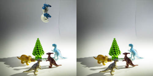
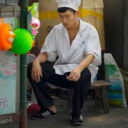
The "smurf removal" above is an example of harmonic inpainting, a method for removing unwanted objects from a photo. Let me stress that the above was not done by Photoshop! Actually Photoshop is the one that uses mathematical techniques.

Harmonic inpainting follows the ideas of Professor Poisson, here depicted among cup lichen (genus Cladonia) using image processing methods based on deep learning:

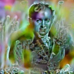
For more information about harmonic inpainting, see this Science SLAM Helsinki video.

One of the important topics in the course is the wavelet transform.

This fall the course concentrates on signal and image processing using matrix methods. The following mathematical techniques will be studied and implemented using Matlab:

• Integration by numerical quadrature,
• Fourier series and Fast Fourier Transform (FFT),
• Wavelet transform, both in 1D and 2D.

We will collect data with smartphone sensors and cameras, and make sense of the data using matrix computations. For example, we will use wavelets for removing noise from the signals and compressing images. There are close connections to JPEG and JPGE2000 image formats, which are based on cosine transform and wavelet transform, respectively.

This course will prepare the students for using computational mathematics both in scientific research and in work life outside the university.

• • News
  • Teaching schedule
  • Exams
  • Course material
  • Registration
  • Exercises
    • Assignments
    • Exercise classes
  • Course feedback

News

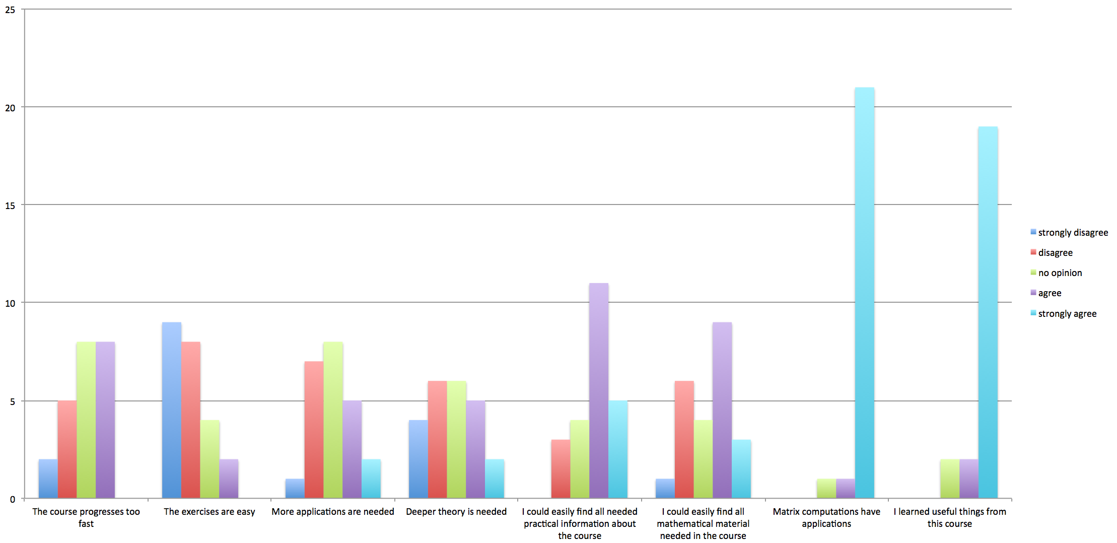
18.10.2016 Results of the feedback questionnaire are in. It seems that the course has been pretty OK:

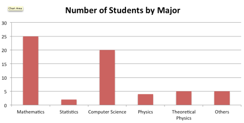
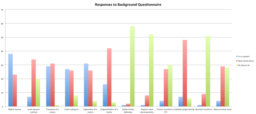
9.9.2016: Results of the background questionnaire are in. This is the distribution of students according to major topic:

Here are the answers to the questions:

Teaching schedule

Weels 36-41, Wednesdays 10-12 and Fridays 12-14 in auditorium CK112. Two hours of exercise classes per week.

Exams

There is no exam. The course is passed by returning answers and solutions to weekly exercises. 

Course material

The course material will be uploaded to this page as the course progresses. The material includes lecture notes and Matlab programs.

Lecture 12 (October 19, 2016)

Experiments with the 2D wavelet transform. Especially: compression of images.

wavetrans2Donce.m, wavetrans2Donce_inv.m, wavetrans2D.m, wavetrans2D_inv.m, Wavelet_tr2D_test.m

Lecture 11 (October 14, 2016)

Explanation of the orthogonal basis of the space L^2([0,1]) provided by Haar wavelets.

Structure of the 2D wavelet transform.

Lecture 10 (October 12, 2016)

Finishing the implementation of the multi-scale wavelet transform. Here are the transform files:

 Wavelet_tr_onestep.m, Wavelet_tr_inv_onestep.m, Wavelet_tr.m, Wavelet_tr_inv.m.

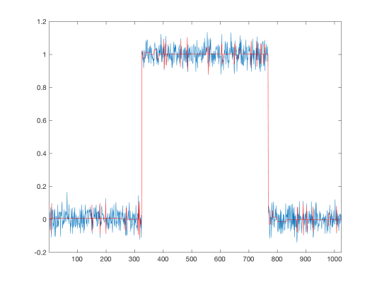
We tested the transform with three different signals:

• Synthetic signal with step discontinuities and added noise,
• Acceleration signal recorded with a smartphone and Matlab Drive (lecture_acc.mat),
• Sound signal recorded in the lecture (Wtrans.m4a, Wtrans.mat).

The signal files are available above. Here is the test routine. 

 Wavelet_tr_test.m

This picture shows the result of noise reduction using Haar wavelets:

Lecture 9 (October 7, 2016)

Programming the one-dimensional multi-scale wavelet transform. It was not quite completed as the multi-scale part of the inverse transform is still in construction.

Wednesday, October 5, 2016: no lecture due to sick leave! 

Lecture 8 (September 30, 2016)

Motivational introduction to wavelets and the amazing Wavelet Transform, both in 1D and 2D. The 2D transform looks like this:

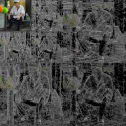
The wavelet transform is useful for removing noise from images as well as for compressing images. The JPEG2000 standard uses wavelets.

Lecture 7 (September 28, 2016)

Complex formulation of Fourier series. See FourierSeries_v1.pdf.

Filtering of signals by setting some of the coefficients to zero (low-pass, high-pass, band-pass filters).

Speeding up the computation by replacing silly for-loops by the legendary Fast Fourier Transform (FFT).

 Fourierseries_complex_test.m, Fourierseries_realsound_test.m (slow with for-loops), Fourierseries_realsoundFFT_test.m (fast with FFT)

The sample sound is available here: testsound.m4a

Lecture 6 (September 23, 2016)

Lecture given by Santeri Kaupinmäki. Topics covered:

• Markov chains
• Ranking webpages (Note: Perron-Frobenius theorem guarantees a unique ranking vector)

Also showed examples of linear regression, markov chain, and webpage ranking in MATLAB.

DataFitExample1.m

TeleOperatorComputation.pdf

TeleOperatorComputation.m

FivePageInternet.m

Lecture 5 (September 21, 2016)

Lecture given by Santeri Kaupinmäki. Topics covered:

• Linear least squares
• Linear regression
• Singular value decomposition (and its application for the minimum norm solution of the linear least squares problem)

The file LeastSquaresStuff_v2.pdfcontains notes on the least squares method and SVD, as well as a proof of the SVD approach to the minimum norm solution in Theorem 4.1.

Lecture 4 (September 16, 2016)
Computational study of Fourier series approximation of functions. Quick conclusions: (1) for a continuous periodic function, a small number of Fourier modes is enough for approximation with high accuracy, and (2) approximating a discontinuous function using Fourier series needs a large number of Fourier modes to avoid "Gibbs phenomenon," or rapid oscillations near the discontinuity. 

 Fourierseries_test.m

Introduction to the source-filter theory of vowel sounds in human speech. Lecture notes (without videos): HumanVoice_v2_share.pdf
For the videos, see https://www.youtube.com/watch?v=Tw2pYY9g6QM 

During the lecture, we recorded the sound of the Electrolarynx, and analysed the signal using Fourier series. Here is the data file and Matlab routine for you to download:

 glottal_excitation.m4a, Fourierseries_glottal.m

Please try the following: approximate the excitation signal using N values 100, 200, 300, 400, 500 and 600. After each computation, listen to the result:

>> sound(sgnl,FS);sound(fseries,FS)

Lecture 3 (September 14, 2016)

Numerical integration using quadrature rules.

• Midpoint rule (essentially the technique discussed in the lecture)
• Trapezoidal rule
• Simpson's rule
• Gaussian quadrature

quadrature_tests.m, gaussint.m (this gaussint.m routine is written by Addie Lambert)

Introduction to Fourier series. Lecture notes: FourierSeries_v1.pdf

Lecture 2 (September 9, 2016)

Opening and saving jpg image files in Matlab. Applying gamma correction to brighten or darken the image.
open_image_in_Matlab.m, gamma_correction.m 

 lecture.jpg

Removing unwanted objects from photographs using harmonic inpainting. Lecture notes: Inpainting_v1_share.pdf

Poisson_FD_solve.m, FD_Laplace.m

 Smurf.jpg

Lecture 1 (September 7, 2016)

Overview of the course
Background questionnaire: Taustatietolomake.pdf
Introduction to applications of matrix computations: CourseIntroduction.pdf; regarding the drum shapes, see
https://www.youtube.com/watch?v=SIOLRcU7FZo 
Case study: X-ray tomography and matrices. See TomographyIntro_v9_share.pdf and the following video:
https://www.youtube.com/watch?v=eWwD_EZuzBI 

Registration

Did you forget to register? What to do?

Exercises

You gain credits from this course only by completing the weekly exercises; there is no exam. Every exercise will have six questions worth six points each. To receive a grade for the exercises send a single pdf-file (no other formats are accepted!) written with your favourite text-editing program and containing your matlab codes (as text), results, images, comments and explanations to the e-mail address application.matrixcomputation@gmail.com by Monday 10 a.m. after the exercise week (for ex. by 10 a.m. on the 19th of September for Exercise 1). Please write the answers in English or Finnish.

Please write in the text of your e-mail which tasks are included in your solution (for ex. Hi! I am sending my solutions to tasks 1, 2, 3, and 5 in the 1st exercise round. Best wishes, Mary Math). Max number of pages is limited to 15. The assistants will not reply to the e-mails; if you have questions related to the exercises, send them as separate e-mails directly to the exercise assistants (usual helsinki.fi-addresses).

 The grading will be decided at the end of the course, but you are guaranteed to pass the course if you get at least 40% of the available exercise points.

The exercise groups are for getting advice from an assistant in solving the exercise problems (participating the exercise class is not obligatory).

The exercise assistants are Santeri Kaupinmäki and Jonatan Lehtonen.

 Results for all exercises (If your results are missing, please contact the exercise assistants by email.)

Exercise06.pdf (Some tips for exercise 1 were added on Monday 17.10.)

wavetrans2Donce.m, wavetrans2Donce_inv.m, wavetrans2D.m, wavetrans2D_inv.m

Exercise05.pdf (Some tips for exercise 1 were added on Friday 07.10.)

Here is material for learning the concept of one-dimensional convolution: Convolution.pdf

 DCT_testing.m, HaarTransform.m, HaarTransformFilter.m, HaarTransformMatrix.m, Tokyo256.mat, TokyoRow.m

Exercise04.pdf  

FFTdemo2D.m

 BigBen.jpg

Exercise03.pdf

kissa.m,DataFitExample1.m

TeleOperatorComputation.pdf

Exercise02_v2.pdf

Ladybug.png

Ladybug2.png

Exercise01.pdf
Note that the biological errors in Problem 6 have been corrected on September 9, 2016! Namely, flies have 5 eyes and rattlesnakes have two horns.
However, if you return an answer to the original form of the exercise, it's OK. 

Assignments

Exercise classes

Course feedback

Course feedback can be given at any point during the course. Click here.