Applications of matrix computations, fall 2015
Applications of matrix computations, fall 2015
Teacher: Samuli Siltanen
Scope: 5 cr
Type: Intermediate studies
Topics: Mathematical modelling using matrices and linear algebra. Many practical applications with a special focus on digital image processing.
Prerequisites: Basic linear algebra. Rudimentary knowledge of Matlab programming is helpful.
Mathematics is applied everywhere in modern life. Whenever you play an mp3 music file, a mathematical algorithm is transforming the zeros and ones in the file into music. Medical CT scans (Computed Tomography) are calculated using mathematical formulas. Washing machines, traffic light control centres, car transmissions and Internet search engines are following sets of mathematical instructions.
It is important to note that the connection between abstract mathematics and the real world is provided by algorithms. Useful mathematics cannot be made only on blackboard, what is needed in addition is programming.
The aim of this course is to train the students in mathematical modelling and problem-solving using algorithms.
Here are some past topics of this course.
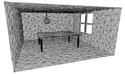
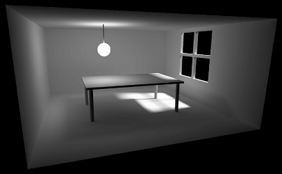
Calculation of lighting for a virtual room using the radiosity method (images by Topi Talvitie):
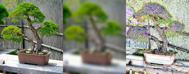
Dividing a photo into its low-frequency and high-frequency components:
Defusing a photobomb (removing an unwanted object from a photo):


Teaching schedule
Weeks 44-49, Wed 10-12 in hall CK112, Fri 12-14 in hall B123 of Exactum. Two hours of exercise classes per week. The course is lectured mainly in English, and the course material will all be available in English.
Lecture on Wednesday, October 28, 2015
Examples of application areas for matrix computations: X-ray tomography, radiosity lighting model, finite element method (FEM) calculations, focus stacking, Google PageRank algorithm.
Slides: , discussion of matrices and X-ray tomography (42MB).
Lecture on Friday, October 30, 2015
Simple example of a system of two linear equations. For the Matlab file, see . Further: we considered an example with three equations for two variables that has no solution, and calculated a least squares solution for it. See the Matlab file . We took a look at the definition of least squares solution and minimum norm solution. Here is some material explaining them: .
Lecture on Wednesday, November 4, 2015
Discussion about least squares solutions. Derivation of the normal equations based on differentiation; here is a and the functional needed therein.
As a specific application we considered fitting a linear model to noisy data, see Chapter 3 in the revised note . Here is the Matlab demonstration routine: . Finally we did a measurement of noisy time-temperature evolution data using an electric kettle.
Lecture on Friday, November 6, 2015
Short discussion about how to organize and sort the electric kettle data from the previous lecture.
Markov chain modeling of simple market share information. See , .
Elementary introduction to Google's PageRank algorithm in a very simple case. , .
Lecture on Wednesday, November 11, 2015
Fourier series in dimension one: an introduction to the world of Fourier techniques. See and the Matlab routine . (In case you are interested in deeper understanding of Fourier transforms and harmonic analysis, the course Fourier Analysis by Professor Kari Astala is highly recommended.)
For a sneak peak on two-dimensional Fast Fourier Transform (FFT) for images, try out the Matlab routine . You will also need the image file .
No lecture on Friday, November 13, 2015
There is a PhD dissertation in the lecture hall, so the lecture is cancelled.
However, there is homework! Please do the following before the lecture on Wednesday, November 18:
(1) Read the Wikipedia entry about Fourier series: https://en.wikipedia.org/wiki/Fourier_series
(2) Take a photograph (with your smartphone or any other digital camera) where something in the picture is in focus and something is not at all in the focus. Here are instructions:
Lecture on Wednesday, November 18, 2015
One-dimensional FFT analysis of the sounds of dialing numbers with a cell phone.
Matlab resources:
Data file, recorded in my office and tapping the phone twice to the table between every number dialling sound:
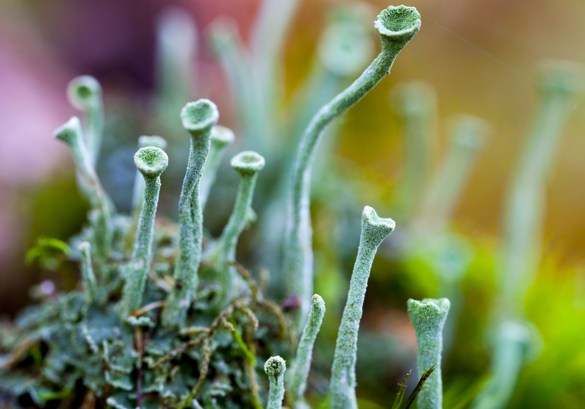
Two-dimensional FFT analysis of an image showing lichen (Cladonia fimbriana). The aim is to divide the image into little patches and analyse the sharpness of each patch separately using FFT.
Matlab resources: , ,
Data file: 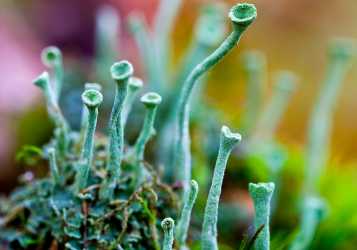
Lecture on Friday, November 20, 2015
Discussion of FFT-based detection of well-focused areas in a photo. Matlab file:
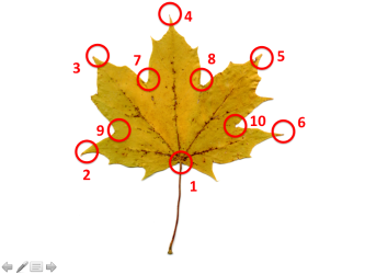
Geometric morphometrics project regarding maple leaves. All students attending the lecture got a dried maple leaf, from which landmark data should be measured. The Matlab file for doing that is here: . The landmarks were agreed to be the ones given in this image:
I kindly ask every student who has a leaf to
(1) scan it,
(2) collect landmark data saved in a file called landmarks.mat, and
(3) send the file to the same email address where the exercises are sent.
Please send the data files at latest during Monday, November 23. Every student who sends such a file on Monday or sooner will get one exercise point.
If you were not in the lecture but would like to take part, you may still find a maple leaf either in a tree or on the ground.
Lecture on Wednesday, November 20, 2015
Procrustes analysis of shapes represented by landmark coordinates.
Here is an explanation how the Procrustes analysis is done in the case of two triangles: .
The related Matlab routine is this: .
This is how the first two of the maple leaf landmark sets look like before and after Procrustes analysis:
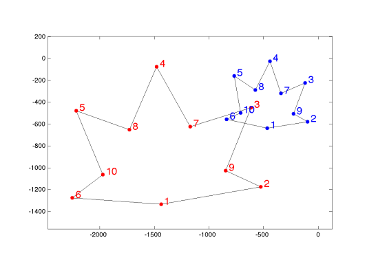
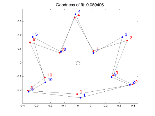
The above images were produced by the Matlab routine when applied to the dataset collected by the students.
(The 16th data of was wrongly input. Exclude this in calculation.)
Lecture on Friday, November 27, 2015.
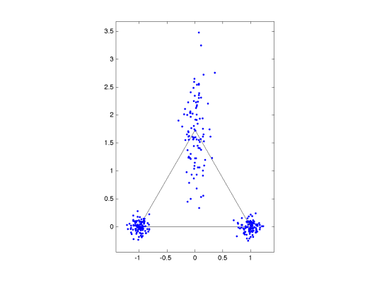
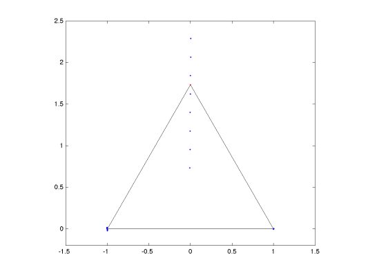
Principal Component Analysis (PCA) as a method of analysing variability in data. We created a simulated dataset of triangles with extra variability in the y-coordinate of the top vertex.
Left image: simulated data. Right: variability among the first principal component.
Matlab files: , ,
Lecture on Wednesday, December 2, 2015.
Finite difference solution method for the Poisson equation. See .
Matlab resources: , .
 Lecture on Friday, December 4, 2015.
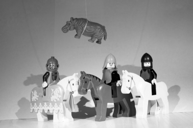

Defusing a black-and-white photobomb, or in other words removing the unwanted hippo from the photograph.
Matlab file:
Image:
Exams
There is no exam, only weekly exercises.
Course material
This course does not follow any specific material. All material needed will be available on this webpage.
If you are not familiar with Matlab, please check out Chapter 1 of http://www.imc.tue.nl/.
Registration
Did you forget to register? What to do?
Exercises
You gain credits from this course only by computing the exercises (there is no exam). There are four simple one-score exercises and two more challenging three-score exercises per week (tentative). To gain the exercise score send a single pdf-file (no other formats are accepted!) written with your favourite text-editing program and containing your matlab codes (as text), results, images, comments and explanations to the e-mail address application.matrixcomputation@gmail.com by Monday 10 a.m. after the exercise week (for ex. by 9th November 10 a.m. for Exercise 1). Please write the answers in English.
Please write in the text of your e-mail which tasks are included in your solution (for ex. Hi! I am sending my solutions to tasks 1, 2, 3, and 5 in the 1st exercise round. Best wishes, Mary Math). Max number of pages is limited to 15. The assistant will not reply the e-mails.
The exercise groups are for getting advice from an assistant in solving the exercise problems. (Participating the exercise class is not obligatory)
The exercise assistant are Zenith Purisha and Topias Rusanen.
Exercise classes
Group | Day | Time | Room | Instructor |
|---|---|---|---|---|
1. | Tuesdays | 12 - 2 pm | C 128 | Zenith Purisha |
2. | Thursdays | 12 - 2 pm | C 128 | Topias Rusanen |
|
|
|
|
|
|
|
|
|
|
|
|
|
|
|
|
|
|
|
|
|
|
|
|
|
Course feedback
Course feedback can be given at any point during the course. Click here.