Applications of matrix computations, fall 2014
Applications of matrix computations, fall 2014
The special focus topic in fall 2014 will be the mathematics of digital image processing.
Lecturer
Scope
5 sp.
Type
Intermediate studies
Prerequisites
Basics of linear algebra (the first year courses Linear Algebra I and II). Some experience with Matlab (or Octave) software is needed.
Lectures
Weeks 44-49 Wed 10-12, Fri 12-14 in hall CK112 of Exactum. Two hours of exercise classes per week. The course is lectured mainly in English, and the course material will all be available in English.
Lecture 1 (October 29,2014):
Introduction to the topic of matrix computations and real-world applications.
Matlab resources:
Images: , , , 

In case you are interested in the radiosity method of computer graphics, you can find the Matlab resources on the Fall 2013 course homepage.
Lecture 2 (October 31,2014):
Visual inspection of linear maps defined by 2x2 matrices using the cat modification algorithm (see kissa.m below).
Quick review of eigenvalues and eigenvectors of matrices, especially in the case of 2x2 matrices.
PageRank algorithm explained in the case of a five-page internet. See .
First connection to importing and handling images with Matlab. Discussion of converting integer pixel values into
floating point values and normalizing pixel values between zero and one.
Bonus material: gamma-correction for a Mars image. You can download the Mars landscape image here; it is also below.
Matlab resources: , , ,
Images: 

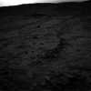 (Mars image copyright: NASA)
Lecture 3 (November 5,2014):
Studying images as continuous and discrete objects. See this note for more details: .The concepts of resolution and downsampling were discussed. Also, Matlab software was created for replacing
a middle part of an image with black color (square and disc areas).
Matlab resources: , , , ,
Images:
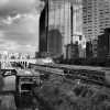 (8bit jpeg version here, for 16bit use load the above file Tokyo2048.tif)
Lecture 4 (November 12,2014):
Discussion of discrete, or quantized, pixel values in images.
Cosine series for even periodic functions. See, for example, http://mathworld.wolfram.com/FourierCosineSeries.html
Matlab resources: , , , .
Lecture 5 (November 14, 2014):
Introduction to the Fast Fourier Transform (FFT) in dimensions 1 and 2.
Matlab resources: , , , , , , ,
Lecture 6 (November 19, 2014)
Low-pass and high-pass filtering of images. Connection between convolution and (fast) Fourier transform.
For the definition of convolution in 1D, please see .
Matlab resources: , , .
Lecture 7 (November 26, 2014)
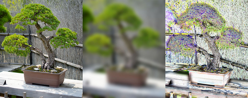
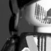
Step towards focus stacking. Choose two sub-images, one with sharp detail and the other one out of focus:
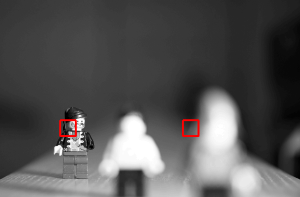

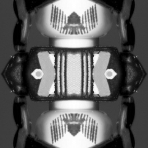
Reflect the two sub-images to enforce periodic boundary conditions for FFT analysis:
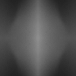
Compare the (logarithms of the absolute values of the) FFTs of these two images:
The left-hand side image window above clearly has a lot more high-frequency content (the red area is wider). This is something that can be detected quantitatively.
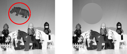
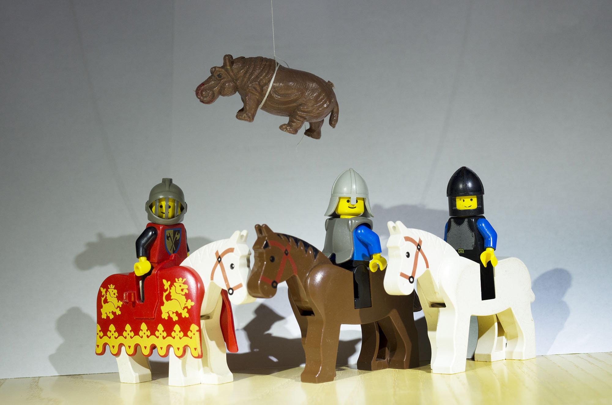
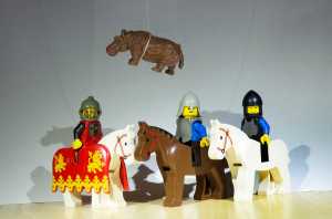
Another topic in this lecture was inpainting, also sometimes known as defusing a photobomb. Suppose we are given an image that has some unwanted element in it, for example a flying hippopotamus. We can surround the area to be removed by a disc, say, and try to use the pixel values at the circle to deduce the missing pixel values inside. Below we show the original image (left, with hippopotamus) and the result (right) of an extremely simple inpainting idea: fill the disc with the average grey level along the circle.
Matlab resources: , ,
Images: ,

Lecture 8 (November 28, 2014):
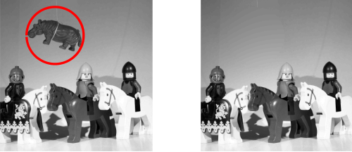
Inpainting topic continued, now actually inserting such grayvalues inside the disc that match the values at the boundary. The motivation for this Poisson-kernel approach comes from physics. If we interpret the pixel values along the boundary of the disc as temperature and the disc as being a metal disc, the temperature evolution inside the disc follows the heat equation. Over time, the temperature will stabilize into an equilibrium state, which in turn satisfies the Laplace equation inside the domain; in other words, the temperature distribution inside the disc is a harmonic function. This is a Dirichlet-type boundary value problem in the field of elliptic partial differential equations (PDE). In this course we do not go into details of PDE theory. Instead, we just use a classical tool from complex analysis called the Poisson kernel. The Poisson kernel can be used to construct a harmonic function inside the unit disc, matching a pre-described boundary value at the unit circle. The boundary value can even be discontinuous.
Here is the result of applying the Poisson kernel:
Another topic in the lecture was X-ray tomography, see .
Matlab resources:
Lecture 9 (December 3, 2014)
Introduction to wavelets, especially the Haar wavelet decomposition and the discrete Haar transform.
Matlab resources: , , , .
More about the topic: Ten lectures on wavelets by Ingrid Daubechies is a great book to read more about wavelets. See also
 Lecture 10 (December 5, 2014)
The Haar wavelet transform for one-dimensional signals at several scales is discussed. A matrix is constructed for realizing the transform.
The 2-D wavelet transform for images was illustrated using Matlab's wavelet toolbox.
Matlab resources: , ,
Exercises
You gain credits from this course only by computing the exercises (there is no exam). There are four simple one-score exercises and two more challenging three-score exercises per week. To gain the exercise score send a single pdf-file (no other formats are accepted!) written with your favourite text-editing program and containing your matlab codes (as text), results, images, comments and explanations to the e-mail address application.matrixcomputation@gmail.com by Monday 10 a.m. after the exercise week (for ex. by 10th November 10 a.m. for Exercise 1). Please write in the text of your e-mail which tasks are included in your solution (for ex. Hi! I am sending my solutions to tasks 1, 2, 3, and 5 in the 1st exercise round. Best wishes, Mary Math). Max number of pages is limited to 15. The assistans will not reply the e-mails.
The exercise groups are for getting advice from an assistant in solving the exercise problems. You can attend any group you like, provided there is room.
The exercise assistants are Tuomas Nikkonen and Zenith Purisha.
Kurssi suoritetaan vain tekemällä harjoitustehtäviä (ei erillistä tenttiä). Kullakin harjoitusviikolla on neljä yksinkertaista yhden pisteen tehtävää ja kaksi haastavampaa kolmen pisteen tehtävää. Tehtäväpisteet saa lähettämällä yhden pdf-tiedoston (ei muita formaatteja!),jonka olet kirjoittanut suosikkitekstinkäsittelyohjelmallasi ja jossa ovat matlab-koodit (tekstinä), tulokset, kuvat, kommentit ja selitykset, osoitteeseen application.matrixcomputation@gmail.com viimeistään harjoitusviikkoa seuraavana maanantaina klo 10 (esim. harjoitukset 1 viimeistään 10.11. klo 10). Laita sähköpostisi viestiosioon tieto siitä, mitkä tehtävät ratkaisit (esim. Hei! Tässä vastaukseni kierroksen 1 tehtäviin 1, 2, 3 ja 5. Terveisin Maija Matikka). Palauta maksimissaan 15 sivuinen raportti. Sähköposteihin ei lähetetä varmistusvastauksia.
Harjoitusryhmissä assistentti neuvoo tehtävien ratkaisemisessa. Voit osallistua mihin ryhmään tahansa, jos huoneessa on tilaa.
Harjoituksia pitävät Tuomas Nikkonen ja Zenith Purisha.
Exercise 1 (November 3-4, 2014)
Exercise 2 (November 10-11, 2014)
Exercise 3
Exercise 4
Exercise 5
Exercise 6
No exercise session on Tuesday 9.12. due to Inversiopäivät conference in Tampere.
Solutions
Grading for Exercise 1 and 2 can be seen at 3rd floor corridor.
Exams
Solving the exercises (no separate exam).
Registration
Did you forget to register? What to do?
Laskuharjoitukset
Ryhmä | Päivä | Aika | Paikka | Pitäjä |
|---|---|---|---|---|
1. | Ma | 12-14 | C128 | Tuomas Nikkonen |
2. | Ti | 10-12 | C128 | Zenith Purisha |