Inversio-ongelmat, kevät 2011
Inversio-ongelmat, kevät 2011
Inverse problems, spring 2011
Finnish summary
Inversio-ongelmien tutkimus on sekä puhtaan että sovelletun matematiikan aktiivinen
osa-alue, joka on Matematiikan ja tilastotieteen laitoksella edustettuna kolmen professorin,
lukuisten tutkijoiden ja jatko-opiskelijoiden sekä Suomen Akatemian huippuyksikön voimin.
Alan tutkimuksessa tavoitteena on saada tuntemattomasta kohteesta tietoa epäsuorien mittausten avulla.
Inversio-ongelmilla on sovelluksia monilla eri tieteen ja tekniikan aloilla.
Näitä ovat mm. signaalinkäsittely, rakenteita tuhoamaton testaus, fysiikka ja astrofysiikka,
muodon optimointi, lääketieteellinen kuvantaminen ja potilaan elintoimintojen seuraaminen,
solubiologia, geofysikaalinen kuvantaminen sekä optiohinnottelu osakemarkkinoilla.
Esimerkkejä inversio-ongelmista:
-Epätarkan valokuvan terävöittäminen
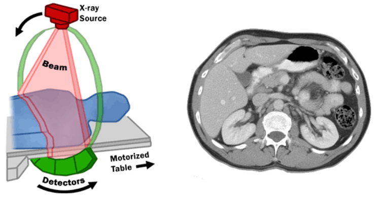
-Kolmiulotteinen röntgentomografia
-Maan rakenteiden kuvantaminen maanjäristysaaltojen kulkuaikojen avulla
-Halkeamien etsiminen rakenteista
-Öljyn ja mineraalien etsintä
-Saasteiden maanalaisen leviämisen havainnointi
-Asteroidien muodon selvittäminen kirkkauden muutosten avulla
Yhteistä kaikille näille ongelmille on niiden herkkyys
mittausvirheille sekä se, että tutkittavasta kohteesta saadaan
vain epäsuoria ja kohinaisia mittauksia.
Keväällä 2011 järjestetään laaja inversio-ongelmien kurssi, jonka
voi sisällyttää sekä yleisen että sovelletun matematiikan syventäviin opintoihin.
Kurssin luennot koostuvat kahdesta osasta:
-Analyyttiset inversio-ongelmat (prof. Matti Lassas)
-Laskennalliset inversio-ongelmat (prof. Samuli Siltanen).
Luentojen laajuus on 5+5=10 op.
Luentojen lisäksi kurssi sisältää aiempaa "Matematiikan sovellusprojektit"-kurssia
vastaavan projektityön. Tämä tehdään ohjattuna parityönä ja sen laajuus on 5 op.
Yhteensä kurssin laajuus on siis 15 op.
English summary
Inverse problems research is an active area of both pure and applied mathematics.
At the Department of Mathematics and Statistics the field is represented by three professors,
several researchers and graduate students and a Centre of Excellence of Academy of Finland.
Inverse problems are about interpreting indirect measurements, and they have
applications to many areas of science and technology. Examples include signal processing,
non-destructive testing, astrophysics, medical imaging and geophysical prospecting.
The lectures of the course consist of two parts:
-Analytic inverse problems (Prof. Matti Lassas)
-Computational inverse problems (Prof. Samuli Siltanen).
Together the lecture parts make up 5+5=10 credit units.
In addition to lectures the course involves a project work. It is done in teams of two and
gives 5 credit units to each student.
The course is in total 15 credit units.
Results
Lecturers
Matti Lassas and Samuli Siltanen
Credit units
15 op.
Type
Advanced studies (syventävä opintojakso)
Prerequisites
Recommended: basics of Fourier transform, measure theory, integration and linear algebra
(for example courses Fourier-muunnoksen perusteet, Mitta- ja integrointiteoria, Lineaarialgebra 1&2).
Experience with Matlab is helpful in the computational part of the course, but not necessary.
Tutorials for learning basics of Matlab are available for example at the following locations:
Lectures
Period III: Lectures and exercises, weekly schedule can be found below.
Tuesday 10-12, hall B120,
Wednesday 10-12, hall B120,
Friday 12-14, hall D123.
Period IV: Project work.
Exam
Friday 15.4, 12-14, hall BK107.
The exam will consists of three problems related to the analytical part of the course
and three problems related to the computational part of the course.
Students need to answer four questions of their choice.
Material
Material for the analytical part of the course will be uploaded here. The material
contains:
Background material 1 (Gunther Uhlmann's lecture notes)
Background material 2 (Guillaume Bal's lecture notes)
Fourier series and Fourier transform Chapters 4 and 9 of Walter Rudin's book Real and Complex analysis
,
.
.
The computational part follows the upcoming book
Linear and nonlinear inverse problems with practical applications
by Jennifer Mueller and Samuli Siltanen. The book will be referred to below as LNIP.
Relevant parts of the book will be copied to the students.
If you need a copy, please come to the lecture or contact samuli.siltanen (at) helsinki.fi.
Also, you can use the old computational . Apart from notation, that document
contains the same concepts and definitions than LNIP.
Sister course
Professor Jennifer Mueller is lecturing a course on inverse problems at Colorado State University (CSU).
She also follows the forthcoming book Linear and nonlinear inverse problems with practical applications,
and the two courses will share software, project topics and other material. Here is the homepage of the
CSU Inverse Problems course.
Matlab files
All Matlab routines given here should be run in a working directory containing a sub-directory called "data".
More precisely: before running the files below, you need to create a subfolder "data" yourself.
Files named as "xxx_comp.m" compute results and save them to sub-directory "data" as .mat -files.
Files named as "xxx_plot.m" read those results from the .mat file and create a plot. This way you can
modify plots easily without repeating possibly time-consuming computations.
One-dimensional deconvolution example:
In the naming convention for Matlab files here, DC stands for "DeConvolution".
Basic routines: , , ,
Simulate continuum data: ,
Create discrete measurement model and test naive inversion including inverse crime.
Experiment with values n=32, n=64 and n=128 in DC_discretedata_comp.m.
, ,
Simulate measurement data avoiding inverse crime. The data is first computed
using a very fine grid to approximate the convolution integral, and then sampled
at k points. Naive inversion is attempted again.
, ,
Truncated SVD (singular value decomposition) is the first noise-robust inversion
method introduced in this course. Here it is applied to the crime-free data computed
in routine DC3_nocrimedata_comp.m. Try the inversion with different resolutions
by running first DC3_nocrimedata_comp.m with n=32, n=64, ..., n=512 and then
running DC4_truncSVD_comp.m.
Tikhonov regularization is a versatile and powerful inversion method. Here are files
for trying out classical Tikhonov regularization with identity matrix in the penalty term,
and also the generalized version with a difference matrix in the penalty term.
Total variation (TV) regularization is the method of choice when edge-preserving reconstructions
are called for. TV-regularized solutions can have jump discontinuities. The following routine makes
use of Matlab's Optimization Toolbox (in particular quadprog.m).
X-ray tomography example (with explicit measurement matrix A):
In the naming convention of Matlab files here, XRM stands for X-Ray tomography with Matrices.
Step A. Create measurement matrices A at different resolutions. The routine XRMA_matrix_comp.m
is not very effective computationally and requires Matlab's Image processing toolbox;
that's why there are a few sample results (.mat files) available below as well. The sample matrices
correspond to measuring NxN images with N evenly spaced angles with N=16,32,50,64.
Copy the .mat files to subdirectory "data" for use.
Step B. Test naive tomographic reconstruction including inverse crime.
Step C. Create tomographic data avoiding inverse crime. This is done by simulating data with
a higher-resolution Shepp-Logan phantom and interpolating the sinogram back to the working resolution.
Due to the special structure of Matlab's radon.m routine, the construction of crime-free data is pretty
complicated. However, you do not need to understand all details of the routine for using it successfully.
This step requires the radon.m function from Matlab's Image processing toolbox, so for
convenience we include some .mat files for those of you who cannot access radon.m.
Step D. Try out naive reconstruction with data from Step C involving no inverse crime.
Step E. Compute singular value decomposition (SVD) of the measurement matrix A. This becomes very
demanding computationally when N is greater than 32.
Step F. Compute regularized reconstructions using truncated SVD. The routine here both computes
the reconstructions and plots them.
Step G. Compute regularized reconstructions with Tikhonov regularization. There is no automatic choice
of regularization parameter here; you can modify the code and experiment with different parameter choices.
Step H. Compute regularized edge-preserving reconstructions using approximate total variation regularization.
The approximation comes from rounding the absolute value function so that the objective functional becomes
differentiable. We use Barzilai-Borwein gradient-based minimization.
The algorithm here includes non-negativity constraint by replacing all negative elements of the iterate by zero
in each iteration. Such box-constrained Barzilai-Borwein method has been analysed by Dai and Fletcher
Numer. Math. (2005) 100. We note that the choice of the initial steplength is done here in a quick-and-dirty way;
it would be more proper to use line search for the first step. These files run and plot the reconstruction:
These files are needed in the working directory when running XRMH_aTV_comp.m:
Schedule
18.1.2011 (Tuesday) Lassas and Siltanen
Introduction to inverse problems, explanation of practicalities of the course.
Introduction to the computational part:
19.1.2011 (Wednesday) Siltanen
Measurement model for one-dimensional convolution and deconvolution,
including continuum integral model and discrete model. See section 2.1 of the book LNIP.
21.1.2011 (Friday) Siltanen
Measurement model for X-ray imaging. Discussion of instability of naive inversion for both
deconvolution and tomography. See sections 2.1 and 2.3 of the book LNIP.
25.1.2011 (Tuesday) Lassas
Models used in analytic inverse problems. We review results on Fourier series.
26.1.2011 (Wednesday) Lassas
28.1.2011 (Friday) Oksanen
Exercise 1, hall D123. Please complete the following 5 problems before the exercise session.
Lauri Oksanen will record which problems the participants have done, and the number of
completed exercises will be taken into account when grading the course.
Problems:
-Exercises 2.4.1-2.4.4 of the book LNIP,
-Study the deconvolution example with Matlab. Find out how low the noise level must be
in routine DC_discretedata_comp.m to give a small error in naive reconstruction.
-Solve the problems in the in the attached
1.2.2011 (Tuesday) Lassas
Lecture
2.2.2011 (Wednesday) Siltanen
Ill-posedness. Singular value decomposition for matrices. Robust inversion using truncated SVD.
4.2.2011 (Friday) Siltanen
Simulation of noisy data. Inverse crime.
8.2.2011 (Tuesday) Lassas
Lecture
9.2.2011 (Wednesday) Siltanen
Tikhonov regularization.
11.2.2011 (Friday) No instruction
If you are not familiar with Matlab, now it's a good time to work through one of the tutorials above.
Also, you might want to familiarize yourself with the X-ray computations given above as they will be
used in the Matlab sessions below.
15.2.2011 (Tuesday) Niemi
Matlab exercise session. It is important to take part; presence in the session affects the course grade positively.
Location: C128.
Create tomographic data with no inverse crime at resolution 16x16 using the routine .
Try naive reconstruction with noisy and non-noisy data.
Compute reconstructions using truncated SVD (you need to write your own m file for this).
Plot the singular vectors and reconstructions as images. Calculate relative errors of reconstructions.
Use filtered backprojection and Tikhonov regularization to recover the 16x16 Shepp-Logan phantom using
and . Compute relative errors.
Which of the above methods gives you the lowest relative error?
Repeat the above computations at resolutions 32x32 and 64x64.
16.2.2011 (Wednesday) Niemi
Exercise session, hall B120.
Problems:
- Exercises 1, 3 and 4 in Section 5.7 of LNIP,
- Solve the problems in the attached
18.2.2011 (Friday) Oksanen
Matlab workshop. It is important to take part; presence in the workshop affects the course grade positively.
Location: C128.
Take the file and make the reconstruction process matrix-free. In other words,
replace all occurrences of matrix A by an application of Matlab's radon.m function and all occurrences
of A^T (transpose of A) by Matlab's iradon.m function with filter choice 'none' (corresponding to unfiltered
backprojection, which is the adjoint of the Radon transform). Push the resolution as high as possible.
Can you reconstruct at 512x512 pixel resolution and 512 angles?
What is the best relative error you can achieve?
22.2.2011 (Tuesday) Lassas
23.2.2011 (Wednesday) Lassas
25.2.2011 (Friday) Siltanen
Idea and definition of total variation regularization. Reformulation as a constrained quadratic optimization
problem. See LNIP, Chapter 6.
1.3.2011 (Tuesday) Siltanen
Large-scale total variation regularization using the rounding trick and gradient-based optimization.
Barzilai-Borwein gradient descent method. See LNIP, Chapter 6.
2.3.2011 (Wednesday) Lassas
4.3.2011 (Friday) Lassas
15.3.2011 (Tuesday) Lassas
16.3.2011 (Wednesday) Lassas Lectures will be held at C123.
18.3.2011 (Friday) There will be no lectures
22.3.2011 (Tuesday) Lassas and Siltanen
Project work topics are chosen. Information about the project work is given. The hall is C123.
Project work
The idea is to study an inverse problem both theoretically and computationally in teams of two students. The end product is a written report consisting of 10-20 pages. We recommend the classical table of contents for structuring the document:
1 Introduction
2 Materials and methods
3 Results
4 Discussion
Section 2 is for describing the data and the inversion methods used. In section 3 those methods are applied to the data and the results are reported with no interpretation; just facts and outcomes of computations are described. Section 4 is the place for discussing the results and drawing conclusions.
First goal: two first sections should be preliminary written. Student A describes the simulation or collection of data, and Student B describes the reconstruction method that will be used. At this point no numerical computations are not necessary. The draft of project work presented at the first deadline will be graded, and the grade represents 30% of the final grade of the project work.
Second and final goal: report is complete. The idea is that Student B simulates or collects the data, and Student B implements the reconstruction.
Topics for project work:
1. Stability and continuity of Radon transform.
The work concentrates on understanding correct function spaces to study Radon transform and its inverse and possibly considering numerical examples. References: Bal's lecture notes, Natterer's book.
2. Acoustic scattering from an obstacle.
The work concentrates on direct and inverse scattering problems and integral equations on the boundary of an obstacle. References: 1. Kress, Linear integral operators, 2. Books of Colton and Kress.
3. Understanding digital filters.
The work concentrates on studying discrete or continuous filters.
4. Inverse problems and Riemannian geometry.
Understanding how geodesic and travel times are related or understanding geometric formulation of inverse conductivity problem. The work is related to invisibility cloaking.
5. Inverse spectral problem or non-linear inverse problem for wave equation.
The work is related to a classical question "Can you hear the shape of a drum?". In the project work one studies one-dimensional spectral problem or one dimensional wave equation and the goal is to understand some of the basic methods how the wave speed can be reconstructed using boundary measurements.
References: 1: Inverse boundary spectral problems (Katchalov-Kurylev-Lassas (Chapter 1), 2: An introduction to inverse scattering and inverse spectral problems (Chadan et al), Chadan's chapter, and 3: An introduction to the mathematical theory of inverse problems (Kirsch, Andreas, Applied Mathematical Sciences, 120. Springer-Verlag, New York, 1996), Chapter 4.
References 1-2 can be found from Kumpulan campus library and reference is provided by the lecturers. More material can be found from American Mathematical Societys web page Mathscinet by searching with words "inverse spectral". In the work one aims to write a report which deals either on the Boundary Control method (Reference 1) or the Gelfand-Levitan method (References 2 and 3).
6. Deblurring a misfocused photograph.
Take a printed paper with some text and an image; a newspaper page will do. Make sure that the page contains a small isolated black dot. It's a good idea to take a sharp picture for comparison and a few misfocused versions with different amount of blur. Also, take photographs with different sensitivities (ISO settings in the camera), resulting in various amounts of measurement noise. Read the photograph into Matlab using the "imread" command and pick out only one of the three color components (red, green or blue). Then you have a grayscale pixel image that can be viewed as a discrete approximation of a real-valued light intensity distribution on the paper. You can read off the shape of the point spread function from the image of the isolated black dot. Apply Tikhonov regularization or (approximate) total variation regularization and find out if you can make the blurred text readable. Read the photograph into Matlab using the "imread" command and pick out only one of the three color components (red, green or blue). Then you have a grayscale pixel image that can be viewed as a discrete approximation of a real-valued light intensity distribution on the paper. You can read off the shape of the point spread function from the image of the isolated black dot. Apply Tikhonov regularization or (approximate) total variation regularization and find out if you can make the blurred text readable.
7. Statistical inversion and Monte Carlo Markov Chain methods
Statistical (Bayesian) inversion provides efficient means for incorporating a priori information into reconstructions. In this project work, one-dimensional deconvolution data is inverted using smoothness requirement (as in generalized Tikhonov regularization with derivative penalty) together with enforcing the information that the signal takes values between zero and one.
8. Wavelets and Besov space regularization
Implement the Besov space regularization method with parameters s=p=q=1 for the one-dimensional deconvolution problem using approximate absolute value function and Barzilai-Borwein minimization.
9. Total variation regularization for tomography
In the lecture material, total variation regularization was implemented for the one-dimensional deconvolution problem using the quadratic programming approach. The aim of this project work is to implement the same approach for the two-dimensional X-ray tomography application.