Radial EIT with the D-bar method
EIT with the D-bar method: smooth and radial case
This page contains computational resources related to the book
Linear and Nonlinear Inverse Problems with Practical Applications
written by Jennifer Mueller and Samuli Siltanen and published by SIAM in 2012.
Return to main page
Introduction
The D-bar method is a reconstruction method for the nonlinear inverse conductivity problem arising from
Electrical Impedance Tomography. This page contains Matlab routines implementing the D-bar method
for a smooth and rotationally symmetric conductivity.
Note carefully that although we use the rotational symmetry of the conductivity to speed up some computations,
the reconstruction process including the solution of the D-bar equation is two-dimensional, not one-dimensional.
Please download the Matlab routines below to your working directory and run them in the order they appear.
Definition of the example
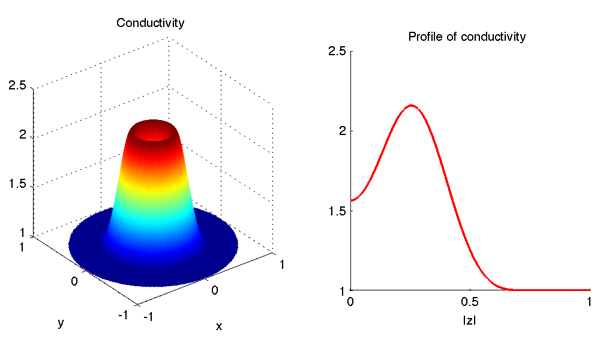
The first example concerns a rotationally symmetric and smooth conductivity that equals one near the unit circle.
Outside the unit disc the conductivity has value 1.
The following file defines a rotationally symmetric and smooth conductivity in the unit disc: .
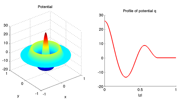
Furthermore, this file implements the Schrödinger potential related to the conductivity: .
The Laplace operator appearing in the definition of the potential is implemented by finite differences in poten.m.
The following routines plot the conductivity and the potential, respectively: , .
Please run the plot commands before continuing to make sure that everything is working properly.
You should see something like this:
Computation of the scattering transform via the Lippmann-Schwinger equation
Next we define a set of points in the k-plane for evaluating the scattering transform t(k).
Because of the rotational symmetry of this example, it is enough to choose k-values along the positive real axis:
the scattering transform is known in this case to be rotationally symmetric and real-valued.
So please download and run this file: .
The above file kvec_comp.m defines a set of k-points and saves them to a file called 'data/kvec.mat'.
(Note that kvec_comp.m creates a subdirectory called 'data'. If you already created it before, Matlab will show
a warning. However, you don't need to care about the warning.)
When running the example for the first time you might just use the file kvec_comp.m as it is.
Later you might want to modify it to choose a different set of k-values.
Now that we have decided on the k-points, it's time to evaluate the scattering transform. Here we do it first by
'cheating', or by knowing the actual conductivity, because then there are no ill-posed steps involved.
Later we will compute the scattering transform also honestly from (simulated) EIT measurements.
This is the file that evaluates the scattering transform t(k) at the k-points: