Colocalization analysis
Before starting a colocalization experiment one should consider what kind of colocalization one hopes to show as the term is poorly defined. Here you can find a simple primer on the topic. Generally colocalization can be defined in three different ways and you should take care to figure out which of the interpretations is applicable to your question. However it is important to remember that this does not prove interaction. Voxels are way larger than proteins even with high magnification objectives and it is possible to have green and red fluorophores in the same 'location' without the proteins / particles being anywhere 'near' each other. FRET experiments can be potentially used to show that the fluorophores are within 10 nm each other this does not directly prove interaction either. It should be noted you should always have a control sample that should yield lower colocalization value that your actual sample. Ideally you would also have positive control. Without the appropriate controls the measured colocalization values mean very little.
Mander's overlap coefficient (MOC)
This parameter tells you simply how large percentage of relevant green signal overlays relevant red signal and the other way around with the signal above the user defined threshold being deemed relevant. In the image below, 100% of the red lies on the green while only 50% of the green lies on the red. So MOC (green, red) = 0.5 while MOC (red, green) = 1. This is very simplistic analysis but if and if you are comparing two or more conditions / samples this method might suffice. Ideally you should have some control samples to give a meaning to your measurements as the numbers themselves might mean very little. 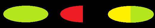
Pearson's correlation coefficient (PCC)
As its name implies, PCC measures how well green and red signal correlate with each other. If the green signal increases as the red signal increases and the red signal decreases when the green signal decreases the signals have high correlation. Correlation coefficient varies from -1 to 1 where minus one implies negative correlation (green where you have no red, red where you have no green), zero means lack of correlation and plus one means perfect correlation. To minimize the impact of background both signals should be thresholded somehow. This means selecting some arbitrary intensity level so that pixels below the level will be disregarded when we calculate the correlation coefficient. However the choice of this parameter introduces bias to the data and no good 'blind' solution exists. Several authors have offered guidelines for the interpretation of a correlation coefficient, but all such criteria are in some ways arbitrary. The interpretation of a correlation coefficient depends on the context and purposes. A correlation of 0.8 may be very low if one is verifying a physical law using high-quality instruments, but may be regarded as very high in the social sciences or in psychological studies where there may be a greater contribution from complicating factors. To solve this problem you must either consult the literature or have a good set of controls so that you can show that your correlation coefficient changes between samples.
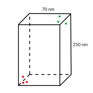
Spot to spot colocalization
As its name implies, the spot to spot colocalization searches for spot-like objects in the sample on two or more channels. The user then defines a distance threshold and the software will tell the user how many green spots are withing the threshold distance of a red spot and how many red sports are within the threshold distance of a green spot. Needless to say this method is only applicable to spot-like objects such as vesicles and nuclei and depends heavily on the quality of the spot detection. If the software cannot detect spots reliably then the analysis will not work. Ideally you should have some control samples to give a meaning to your measurements. The fact that 60% of the green dots are within 500 nm of red dots might not mean much without proper controls or relevant literature references. 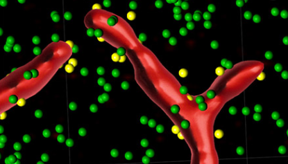
results from BISE
Frequently used at HELMI
https://biii.eu/2-d-colocalisation-cells
https://biii.eu/cellprofiler-examples-colocalization
https://biii.eu/spot-detection-and-codistribution-analysis
Examples from HELMI