Viscous flow in Python

Overview

As we’ve seen previously, most landforms on Earth are sculpted by the flow of fluids across the landscape. Erosion by glaciers can significantly change the Earth’s surface, moving vast quantities of material from high elevations to lower elevations. Glacial landscapes are unique and clearly reflect erosion by processes that differ greatly from those found in fluvial systems. To understand how material is moved within glacial systems, it is important to first understand the dominant controls on glacier velocities.

Non-Newtonian flow in open channels

Background

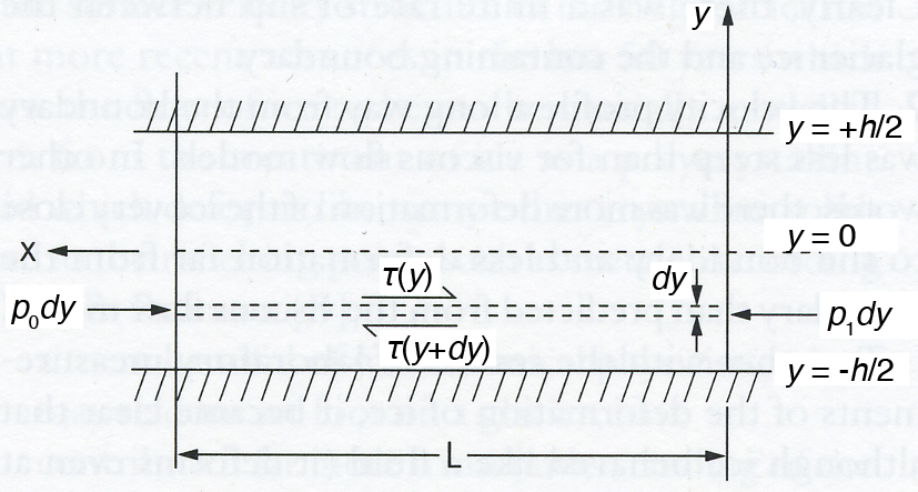Figure 1. Schematic diagram of pressure-driven flow in a channel.

The viscosity of ice depends on both temperature and stress. For simplicity, we’ll consider the case where viscosity is only a function of shear stress. Consider a channel of width h centered about y = 0, with lateral boundaries at y = ±h/2 (Figure 1). A pressure gradient Δp = p₁ - p₀ drives flow within the channel of length L.  The shear stress in the fluid depends on the applied pressure gradient and the distance from the channel boundaries

where τ is the shear stress. We know that for Newtonian fluids

where η is the dynamic viscosity of the fluid. Substituting the right side of Equation 2 into the left side of Equation 1 we find

Integrating Equation 3 twice we get

Since we know du/dy = 0 at y = 0, we find c₁ = 0, and because we assume zero slip at the boundaries of the channel (u = 0 at y = ±h/2), c₂ = (1/2η)(dp/dx)(h/2)². Thus,

This is the velocity profile for a Newtonian fluid, but as you will recall, we learned that ice is a non-Newtonian (nonlinear viscous) fluid. As such, the behavior should be modeled using a power-law, where the strain rate is a related to the shear stress as follows

where a is a function of the viscosity and temperature (we will ignore temperature for now), and n is the power-law exponent. If we solve Equation 7 in terms of τ, we can substitute the result into Equation 1 to get

Assuming symmetry about the center line, y = 0, and integrating we see

Now integrate Equation 9 and assume u = 0 at y = ±h/2

The mean velocity in the fluid is

We can calculate a non-dimensional velocity now by dividing the velocity at any point in the channel by the mean velocity

Exercise 1 - Planform flow velocity across a glacier

Files for this exercise

• open_channel_ex1.py
• sask_glacier_ex1.py
• sask_glacier_velo.txt

The goal of this exercise is to calculate horizontal velocity profiles across a glacier for Newtonian and non-Newtonian fluid flow resulting from a pressure gradient.

1. Modify the Python script file open_channel_ex1.pyto plot the non-dimensional velocity (u/u̅) of a fluid as a function of non-dimensional distance (y/h) across the channel of width h (Equation 12). Assume the flow is symmetrical about y = 0 and the velocity is zero at the boundaries of the channel. In your Python script you should

   1. Solve for the non-dimensional velocity across the channel for a Newtonian fluid and for non-Newtonian fluid with power-law exponents of n = 2, 3, 4, 5

      The flow is symmetric about y = 0 and for negative y values the equation does not work properly. You can solve one half of the flow (y ≥ 0) and use symmetry to plot the other half of the flow.

   2. Create one plot of the non-dimensional velocity of all of the fluids as a function of non-dimensional distance.
      1. Be sure to label your axes and add a title
      2. Also include text labels beside each velocity profile listing the power-law exponent
      3. How sensitive is the velocity to the power-law exponent? What is the maximum percent difference in velocity between n = 2 and n = 4?
   3. Include clear comments that explain what each section of your code does

2. The Saskatchewan glacier near Banff in Alberta, Canada (Figures 2-4) is 1400 m wide and part of a large ice field known as the Columbia Icefield.
   
   
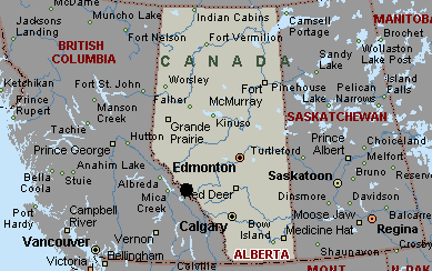
   Figure 2. Map of western Canada with the location of the Saskatchewan glacier in Banff, Alberta indicated with a filled black circle.   
   (Source: Microsoft MapPoint 2004)
   
   
   Figure 3. Topographic map of Saskatchewan glacier.   
   (Source: http://earth.esa.int/workshops/fringe_1996/cumming/loadmap.htm)
   
   
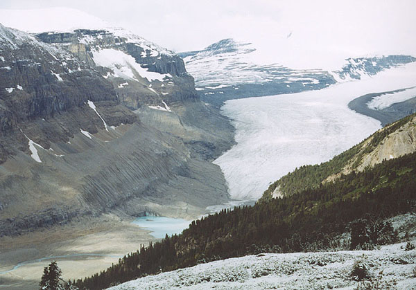
   Figure 4. Saskatchewan glacier from Parker Ridge.   
   (Source: http://www.giorgiozanetti.ca/rockies_2002/banff_large.html)
   
   

   	Velocity
   Distance from center line [m]	[m/a]	[m/s]
   -660	12	3.80E-07
   -640	22	7.00E-07
   -570	42	1.33E-06
   -460	63	2.00E-06
   -220	74	2.35E-06
   40	76	2.41E-06
   180	74	2.35E-06
   260	72	2.28E-06
   500	51	1.62E-06

   Table 1. Velocity measurements across the Saskatchewan glacier.
   
   The file sask_glacier_velo.txtcontains a series of surface velocities measured at various locations across the glacier (Table 1). Modify the Python script sask_glacier_ex1.pyto plot the measured velocities as a function of distance from the center line of the glacier, and also plot predicted velocity profiles for several non-Newtonian fluids (Equation 10). Assume a = 5 × 10^-24 Pa^-3 s^-1. In your program you should

   Solve for the velocity profile of a non-Newtonian fluid with power-law exponents of n = 2, 3, 4, 5

   The term (p₁ -p₀)/L in Equation 10 is an unknown. However, you can solve for it using the condition that the maximum flow velocity (~2.41 × 10^-6 m/s) occurs at y = 0. Once you have solved for that term, you can insert it back into Equation 10 to solve for the velocities elsewhere.

   Again, the flow is symmetric about y = 0 and for negative y-values Equation 10 does not work properly. Use the symmetry of the solution to make your plot.

   1. Load the observed velocity data
   2. Plot the measured velocities along with the 4 predicted velocity profiles. Be sure to label your axes and include a title. Also include text labels beside each velocity profile listing the power-law exponent.
   3. Include clear comments explaining what each section of the code does.

For exercise 1 you should submit

1.  2 Python plots
   1. Non-dimensional velocity profiles for Newtonian and non-Newtonian fluids (Part 1 above)
   2. Velocity profile across the Saskatchewan glacier with points showing the measured velocities (Part 2 above)
2. Copies of your modified Python scripts that produce the plots
3. Figure captions for each plot describing the plot as if it were in a scientific journal article.
   1. For the second plot, list the most likely power-law exponent n for the Saskatchewan glacier in the caption text

Non-Newtonian flow down an inclined plane

Background

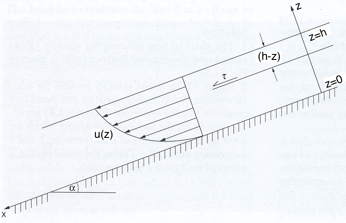Figure 5. Schematic diagram of a viscous fluid flowing down an inclined plane.

The velocity of a fluid flowing down an inclined plane can be modelled using some basic physical relationships. First, recall that the basal shear stress for a fluid flowing down an inclined plane is due to the down slope component of the weight of the overlying fluid

where ρ is the fluid density, g is the acceleration due to gravity, h is the thickness of the fluid perpendicular to the inclined plane and α is the angle of the plane with respect to horizontal. At any distance z above the bed

where γ_x = ρgsin(α) is the downslope component of the gravitational force. Combining Equation 2 with Equation 14 we find the constitutive equation for a Newtonian fluid is

Integrating Equation 15 yields

where c₁ = 0 from the boundary condition u = 0 at z = 0. Equation 16 can be rewritten as

For a non-Newtonian fluid, Equation 14 can be modified to account for the case where the strain rate varies as a power of the shear stress (Equation 7)

To determine the velocity profile, we need to integrate Equation 18. If we use the boundary condition that the basal sliding velocity is equal to u_b rather than zero, we get

Exercise 2 - Vertical velocity profile in a glacier

Files for this exercise

• atha_glacier_ex2.py
• atha_glacier_velo.txt

The goal of this exercise is to calculate vertical velocity profiles across a glacier for Newtonian and non-Newtonian fluid flow resulting from a gravitational forces on the glacier.

1. The Athabasca glacier (Figures 6, 7) is another glacier in the Columbia Icefield (see Figures 2, 3 for location).
   
   
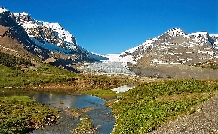
   Figure 6. Athabasca glacier landscape.
   (Source: http://www.pbase.com/image/27382295)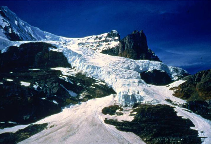 
   
   
   Figure 7. Athabasca glacier landscape.
   (Source: http://www.canadianheritage.org/reproductions/23026.htm)

   Depth from surface	Height from base z	Horizontal velocity
   [m]	[m]	[m/a]	[m/s]
   0	209	28.6	9.10E-07
   15	195	28.5	9.00E-07
   30	180	28.5	9.00E-07
   45	165	28.4	9.00E-07
   60	150	28.2	8.90E-07
   75	135	28.0	8.90E-07
   90	120	27.7	8.80E-07
   105	105	27.2	8.60E-07
   120	90	26.5	8.40E-07
   135	75	25.5	8.10E-07
   150	60	24.0	7.60E-07
   165	45	21.5	6.80E-07
   180	30	17.5	5.50E-07
   195	15	10	3.20E-07
   209	0	4	1.30E-07

   Table 2. Velocities measured from a vertical profile through Athabasca glacier.
   
   A vertical velocity profile for the Athabasca glacier has been measured and the measurements are in the file atha_glacier_velo.txt(Table 2). Modify the provided Python script atha_glacier_ex2.pyto plot the velocity measurements (x-axis) versus the height (z-axis) from the bed. On the same plot, include Newtonian and non-Newtonian fluid flow profiles as well (Equation 19). Assume a = 5 × 10^-24 Pa^-3 s^-1. In your code, you should

   Solve for the velocity profile for a Newtonian fluid. Your profile should have a no-slip basal boundary condition (u_b = 0) and honor the observed surface velocity.

   Again, in this problem there is an unknown term γ_x in Equation 19. However, you can solve for it using the condition that the maximum flow velocity (~0.91 × 10^-6 m/s) occurs at z = h = 209 m. Once you have solved for that term, you can insert it back into Equation 19 to solve for the velocities elsewhere.

   1. Solve for the velocity profiles of non-Newtonian fluids with power-law exponents of n = 2, 3, 4, 5 (Equation 19). You should set u_b equal to the observed value (Table 2) and your Python program should honour the observed surface velocity (see tip above)
   2. Load in the observed velocity profile data
   3. Generate a plot of the observed velocity values, the predicted Newtonian velocity profile and the 4 non-Newtonian velocity profiles
   4. Include clear comments that explain what each section of the program does

For Exercise 2 you should submit

1. One Python plot of the Newtonian and non-Newtonian velocity profiles across the Athabasca glacier with data points showing the measured velocities
2. A copy of your Python script that produces the plot
3. A figure caption for the plot describing the plot as if it were in a scientific journal article.
   1. In the caption you should list the most likely value for the power-law n exponent for the Athabasca glacier.