Thermochronology in Python II

Overview

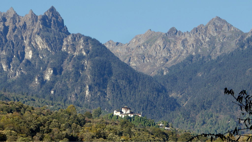
The Himalaya in Bhutan (click to enlarge). Image source.

The overall goal of this exercise is to interpret a thermochronometer dataset from the Himalaya of Bhutan. The interpretation entails determining long-term average rock exhumation rates from rock samples analyzed using apatite and zircon (U-Th)/He and muscovite ⁴⁰Ar/³⁹Ar thermochronology. As you will recall, our exercise last week used a simple 1-D transient solution to the advection-diffusion equation to calculate a temperature-depth profile in the Earth, which was then used to predict thermochronometer ages based on Dodson's method. In that model, we specified a rock exhumation rate and observed variations in the thermochronometer ages as a function of exhumation rate. This week, we will compare those predicted thermochronometer ages to data from Bhutan with the goal of minimizing the misfit between the measured and predicted thermochronometer ages by varying the specified rock exhumation rate, which will allow us to define a best-fit exhumation rate (or exhumation history) for the Himalaya of Bhutan. For this exercise, we will be using data from Coutand et al., 2014 and Stüwe and Foster, 2001.

Exercise 1 - Comparing measured and predicted thermochronometer ages, again

Files for this exercise

• age_predict_1D.py
• Bhutan_age_data.txt

In order to be able to compare our predicted thermochronometer ages to some data, we'll first need to load the data file. You are welcome to use the example script file above to make your modifications (I have noted where to make changes), but it might be better to copy your Python script from last week and make changes to that code.

1. Using the past exercises as examples (look at those codes ), you should add code to bottom your Python script (after the predicted thermochronometer ages are calculated) to read a data file and store the contents in different variables in the code. The data file has a header that lists the data contained in each column. You may want to look at the data file in a text editor in order to give logical names to the variables in the data file.

2. Once you have added the code to read the data file, you will want to calculate goodness-of-fit values for each thermochronometer system, as well as a total goodness-of-fit value for all of the age data. You should use the same goodness-of-fit equation we have used in the previous exercises, and be sure to divide the goodness-of-fit value by the number of measured ages for each thermochronometer. The goodness of fit equation you should use is

   Unknown macro: mathdisplay. Click on this message for details.

   The [mathdisplay] macro is not in the list of registered macros. Verify the spelling or contact your administrator.

   where n is the number of ages, O_i is the ith measured age, E_i is the ith predicted age and σ_i is the ith standard deviation.

   Be aware that measured ages are listed for each sample location in the data file, but not every sample has been analyzed for each different thermochronometer system. Thus, there are ages of '-9999' listed in the data file. Those ages are listed there to indicate there is no corresponding measured age for that thermochronometer system at that sample location. Those ages should be ignored in your goodness-of-fit calculation using an if statement.

3. The last task is to produce a useful plot. For this, we will again use the subplot() command to make a plot that shows (1) the predicted geotherm and particle temperature-depth history in the upper panel (i.e., the plot from Laboratory Exercise 6), and (2) the predicted and measured age data on the lower panel.

   For the lower plot, the x-axis should plot latitude and the y-axis should plot thermochronometer age, including error bars for the measured ages.

   It may help to plot the different thermochronometer systems with different color symbols.

   The predicted ages can be shown using lines of constant age that have a range that includes the entire range of latitude of the measured age data.

   This plot should also list the goodness-of-fit values for each thermochronometer system, as well as the total goodness-of-fit for the age dataset.

For this exercise, submit a copy of your Python code and the plot you produce for point 3 above with an advection velocity of 0.5 mm/a. Include a descriptive figure caption as well.

Exercise 2 - "Fitting" thermochronometer data

Using the modified Python script above, you goal is now to find an average long-term exhumation rate that provides a good fit to the measured thermochronometer data.

1. Comparing the goodness-of-fit values and the plotted age data, run a series of models in which you only change the vertical advection velocity (exhumation rate) in order to find a minimum goodness-of-fit value for the whole thermochronometer age dataset. You do not need to find the absolute minimum goodness-of-fit value, but rather a value that is the minimum at an exhumation rate of v_z ± 0.2 mm/a. Save a copy of this plot for your report and be sure the advection velocity (exhumation rate) and misfit value are clearly displayed.
2. Now take an alternative approach and minimize the goodness-of-fit values for each individual thermochronometer system (e.g., apatite (U-Th)/He goodness-of-fit, zircon, muscovite). As above, you do not need an absolute minimum misfit value, but one that does not decrease in the range v_z ± 0.2 mm/a. You should save a copy of each plot with the minimum goodness-of-fit displayed for each thermochronometer along with the exhumation rate. You do not necessarily need to include all of these plots in your report, but you may want to include some of them.

For this exercise, submit a copy of each of the plots you produce above (4 in total) and provide a descriptive figure caption for each figure.

References

Coutand, I., Whipp, D. M., Grujic, D., Bernet, M., Fellin, M. G., Bookhagen, B., et al. (2014). Geometry and kinematics of the Main Himalayan Thrust and Neogene crustal exhumation in the Bhutanese Himalaya derived from inversion of multithermochronologic data. Journal of Geophysical Research: Solid Earth. doi:10.1002/2013JB010891

Ehlers, T. A. (2005). Crustal Thermal Processes and the Interpretation of Thermochronometer Data. In P. W. Reiners & T. A. Ehlers (Eds.), Low-Temperature Thermochronology: Techniques, Interpretations and Applications (Vol. 58, pp. 315–350). Mineralogical Society of America.

Reiners, P. W., & Brandon, M. T. (2006). Using Thermochronology to Understand Orogenic Erosion. Annual Review of Earth and Planetary Sciences, 34, 419–466.

Stüwe, K., & Foster, D. (2001). ^{4039Ar/Ar, pressure, temperature and fission track constraints on the age and nature of metamorphism around the main central thrust in the eastern Bhutan Himalaya}. Journal of Asian Earth Sciences, 19(1), 85–95.