Advection processes in Python

Overview

For the exercises this week, we will be applying the advection equation to bedrock river erosion with a spatially variable advection coefficient (stream-power erosion). 

You are asked to modify an existing Python script to produce plots and to answer questions related to the plots. As before, we will be using Canopy for these exercises.

Exercise 1 - Introduction to river profile evolution

File(s) for this exercise

• Python script for Exercise 1

For this exercise we will be using the Python script river_profiles_ex1.pyto plot river profiles. The script performs all of the basic calculations needed to answer the questions below, but you will be required to make some changes to the script to complete the exercise. To begin, make a new directory on the Desktop for this week's exercise (e.g., QG-Lab4), copy the river_profiles_ex1.py file to that directory and open it in the Canopy editor.

1. The program simulates river incision into a 100-km-wide landscape with an initial flat surface elevation of 1500 m. River incision is calculated using the stream-power erosion equations described in Lecture 7. For this part you should do the following:1. Carefully read over the Python source code and comments. There are some new features in this code, so pay attention to where the variables are defined and used, how the initial topography is defined, how the upstream drainage basin area is calculated, how surface elevation is calculated and how the results are plotted.

   1. Without making any changes, run the program and save a copy of the plot it produces. The program will take about 1 minute to run. Insert the plot into your write-up for this week's exercises and add a figure caption explaining what the plot shows.

   2. Look again through the Python code and the plot it produces. Answer the following questions in the space below the plot and caption you've inserted previously.* How long is the time step in the calculation?

      • What is the rock uplift rate in the model? Is it constant or does it vary with space in the model?

      • What is the maximum elevation of the topography at the end of the simulation? Is this higher or lower than the original maximum elevation? Why?

      • Does the maximum elevation continually increase with time, or does it also decrease? Why might this be? Does the river profile appear to reach a steady state?

      • How fast (at what velocity) does the drainage divide (highest point in the topography) migrate across the model? To calculate this value, you should run the model several times for shorter simulation times, note the position of the divide at the completion of the simulation and then calculate the velocity (distance travelled divided by time).

2. This program calculated erosion rates across the length of the channel as a function of time in order to update the topography at the end of each time step. Currently, the program only plots the topography. For this part of the exercise, your goal is to plot both the topography and erosion rates on separate plots. This can be done using the plt.subplot() function to add a second plot, similar to what is currently done for plot 1. Currently, plot 1 is created in the Python script using the commands

   # Format subplot 1
   axis1 = plt.subplot(1,1,1)                  # Set axis1 as the first plot
   axis1.set_xlim([0.0, max(xkm)])             # Set the x-axis limits for plot 1
   axis1.set_ylim([0.0, max_elevation*1.1])    # Set the y-axis limits for plot 1
   plot1, = plt.plot(xkm, topography)          # Define plot1 as the first plot
   plt.xlabel("Distance from drainage divide [km]")
   plt.ylabel("River channel elevation [m]")
   plt.title("River channel profile evolution model")

   This is slightly different than past plots for two reasons. First, we would ultimately like to have multiple plots in one window. Second, to update the plot in an animation in the plot window, we need to define a variable to refer to the plot frame (axis1) and the line that will be plotted (plot1). Here, by using plt.subplot function, we have allowed ourselves to have several plots in one window. The syntax for the plt.subplot command is plt.subplot(nrows, ncols, plot number), where nrows is the number of rows of plots, ncols is the number of columns of plots and plot number is the number of the plot in the list. Currently, we have 1 row, 1 column and 1 plot to display. Note that we have also defined the axis limits separately so they can be updated in the animation. For this part, you should

   First increase the number of rows to two for the first plot, then add the code necessary to generate a second plot similar to the example for plot 1. The second plot should be below the first plot and show the erosion rate in mm/a across the river profile with proper axis labels.

   Because the coordinate system for elevation is positive upwards, you should multiply the erosion rates that are calculated by -1 so that they are positive values.

    If you run your simulation for 100,000 years, you should see something like the following plot:
   

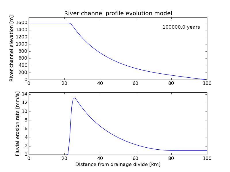
   Add your plot to your write-up and give it a descriptive figure caption.

   1. Run the program with a rock uplift rate of 1 mm/a and answer the following questions in your write-up:
      • What are the fastest erosion rates your see in your river profile?
      • Do the fastest erosion rates always occur in the same place, or does the location of fastest erosion change? Explain why this occurs, based on the equations for stream-power erosion presented in Lecture 7.
   2. Rerun the program with a rock uplift rate of 3 mm/a and answer the following questions in your write-up:

   What is the maximum elevation you observe in the model after 100,000 years now?

   1. 
      
      • What is the maximum erosion rate in the model after 100,000 and 2,000,000 years? Does the river profile reach an equilibrium elevation?
3. Modify the program so that it now uses an initial topography that is sloping, rather than flat. This feature is already available in the code, but you will need to locate it and change the corresponding variable in order to use sloping initial topography. Rerun the program and perform the following steps:
   1. Save the plot that is generated after 2,000,000 years with a rock uplift rate of 1 mm/a, insert it into your write-up and add a descriptive figure caption.
   2. Explain how fast (at what velocity) the drainage divide migrates back into the initial topographic surface. As before, you may want to run several shorter simulations to calculate the position of the divide at various times in order to find a velocity (distance over time). How fast is this velocity compared to that calculated in question 1?
   3. Look at the erosion rates across the profile. Are the majority of the erosion rates greater than, less than or equal to the rock uplift rate? Based on this answer, is the topography in a steady state (i.e., not changing)?
4. Change the initial topography back to a flat surface. In the stream-power erosion law, there are two important exponents (m and n) that will alter the efficiency of river erosion when varied. Change the values of m and n to the different values listed in the comments in the code and rerun the program for each pair of m and n values.
   1. Save a copy of each plot that is generated and add a descriptive figure caption in your write-up.
   2. Is the river channel profile sensitive to variations in m and n?
5. Change the values of m and n back to the original values (m = 1.0, n= 2.0). Currently, the program uses a constant rock uplift rate across the river profile. Modify the program to have a rock uplift rate of 5 mm/a when x ≤ 50 km, and an uplift rate of 1 mm/a when x > 50 km. This discontinuity is equivalent to placing an active fault along the river profile. Rerun the program and perform the following tasks:
   1. Save a copy of the plot that is generated and add a descriptive figure caption in your write-up.
   2. Answer the following questions:
      • Is the maximum topography higher or lower in this simulation compared to that in question 1?
      • Does the river profile after 2 million years clearly show where the change in uplift rate occurs?
      • Does the plot of erosion rates clearly show where the change in uplift rate occurs as the profile evolves?

For this part of the exercise, you should submit a Word document or PDF with

1. All of the requested plots from the previous questions, descriptive figure captions for each plot and answers to any related questions.
2. A copy of your modified Python code from question 5 either copied and pasted into the end of your write-up, or as a separate document uploaded to Moodle.